Page 381 - Fundamentals of Water Treatment Unit Processes : Physical, Chemical, and Biological

336 Fundamentals of Water Treatment Unit Processes: Physical, Chemical, and Biological

operation. Theory provided the rationale for the excursions where
from standard designs and pilot plants provided the empirical C is the concentration of suspended matter of a given
3
confirmation. species (kg suspended solids=m of water)
3
s is the specific solids deposit on media (kg of solids=m of
12.3 THEORY total volume of filter)
i is the local hydraulic gradient (m headloss=mof filter
Experimental work aimed at discovering filtration mechan- depth)
isms started with Eliassen (1941) reporting on doctoral Z is the coordinate distance in vertical direction (m)
research completed at MIT in 1935, followed by Stein t is the elapsed time since introduction of suspended matter
(1940), Stanley (1955), and Ives (1961,1962). Filtration the- to filter medium (s)
ory, in the mathematical modeling sense, started with a paper
by Iwasaki (1937) (Section 12.3.3.1). Ives (1962) coupled his The three functional relations are aspects of the same
experimental work with mathematical modeling, building on phenomenon, that is, the loss of a portion of the suspended
Iwasaki’s work. solids from suspension within the pores of the filter bed, and
their subsequent deposit on the grains of the filter medium,
and the ‘‘clogging’’ of the medium that causes increase in
12.3.1 QUEST OF THEORY
hydraulic gradient.
Goals of filtration theory are as follows: (1) to describe vari-
ables that affect particle removal, (2) to develop mathematical 12.3.1.2 Definitions
models that describe filtration behavior, and (3) to explain the
The C(Z) t curve is called here the ‘‘wave front’’; the C(t) Z
mechanisms of particle removal in depth filtration. Issues curve is called the ‘‘breakthrough’’ curve; the two curves are
include the rate of clogging, the rate of headloss increase, related mathematically. The s(Z) t curve is the ‘‘clogging-
effluent particle counts with time, backwash effectiveness, etc. front.’’ The hydraulic gradient profile, i(Z) t is related to the
clogging-front, which is also related to the wave front.
12.3.1.1 Dependent Functions in Filtration
In filtration, the suspended solids concentration and the
deposited solids both change with depth and with time. At 12.3.2 PROCESS DESCRIPTION
the same time, the local hydraulic gradient changes with Several experimental investigations have provided data that
distance and time due to the continuing depositing of solids describe the filtration process in terms of C(Z, t) results.
along the depth of the filter column. The respective functional
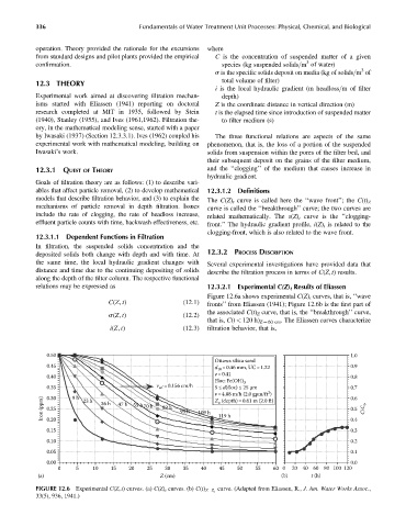
relations may be expressed as 12.3.2.1 Experimental C(Z) t Results of Eliassen
Figure 12.6a shows experimental C(Z) t curves, that is, ‘‘wave
C(Z, t) (12:1) fronts’’ from Eliassen (1941); Figure 12.6b is the first part of
the associated C(t) Z curve, that is, the ‘‘breakthrough’’ curve,
s(Z, t) (12:2)
that is, C(t < 120 h) Z ¼ 60 cm . The Eliassen curves characterize
i(Z, t) (12:3) filtration behavior, that is,

0.50 1.0
Ottawa silica sand
0.45 d =0.46 mm, UC=1.22 0.9
10
e=0.41
0.40 0.8
Floc: Fe(OH) 3
0.35 v =0.156 cm/h 5 ≤ d(floc) ≤ 25 μm 0.7
wf
2
v =4.88 m/h (2.0 gpm/ft ) 0.6
9 h
0.30
Iron (ppm) 0.25 36 h 47 h 55 h 70 h 82 h 95 h 109 h Z o 119 h 0.5 C/C o
(depth)=0.61 m (2.0 ft)
23 h
0.20
0.3
0.15 0.4
0.10 0.2
0.05 0.1
0.00 0.0
0 5 10 15 20 25 30 35 40 45 50 55 60 0 20 40 60 80 100 120
(a) Z (cm) (b) t (h)
FIGURE 12.6 Experimental C(Z, t) curves. (a) C(Z) t curves. (b) C(t) Z¼Z o curve. (Adapted from Eliassen, R., J. Am. Water Works Assoc.,
33(5), 936, 1941.)