Page 386 - Fundamentals of Water Treatment Unit Processes : Physical, Chemical, and Biological

Rapid Filtration 341

30 345 30
v(clogging front) ≈ 3.0 cm/210 min
= 0.014 cm/min = 0.86 cm/h 320
25 280 25
Clogging front 240 20
Headloss (cm of water) 15 70 200 Total headloss at Z = 20 cm (cm water) 15 Clean-bed headloss
20

135

10
0 min 40 10
5 5

0
0
0 5 10 15 20 0 50 100 150 200 250 300 350
(a) Z (cm) (b) Time (min)

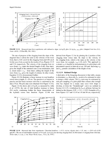
FIGURE 12.13 Measured data from experiments with radioactive algae. (a) h L (Z) t plot. (b) h L (t) Z ¼ 20cm plot. (Adapted from Ives, K.J.,
Trans. ASCE, 127(Part III), 384, 1962.)

The rate of progress of the clogging front (the slope of the derived from Figure 12.14a by plotting the Z position of the
diagonal line) is about the same as the velocity of the wave clogging front versus time. Its slope is the velocity of
front, that is, 0.84 cm=h for the clogging front and 0.90 cm=h the clogging front, which is the same as the velocity of the
for the wave front, as seen by the results of Ives, Figures 12.15 wave front, for example, v wf 2.8 cm=h. This approach to
and 12.9, respectively. The velocity of the clogging front (or evaluate v wf is feasible by instrumentation of a pilot plant with
wave front), v wf , times the desired length of run, t(run time), piezometers spaced at intervals at say 100 mm. Knowing v wf
gives the length of the saturated zone at run termination, that and L wf permits calculation of the length of run.
is, (L(sat zone) ¼ v wf t(run time); adding the length of the
wave front, L wf , gives the length of column. In other words, 12.3.2.9 Rational Design
Equation 12.10 is demonstrated further. A derivative of the foregoing discussion is that with a means
Figure 12.13b illustrates a linear increase in total headloss to determine v wf , then only L wf needs to be estimated in order
versus time at depth, Z ¼ 20 cm. The question is of interest in to design a filter column. The L wf term may be estimated by
practice and the linear increase with time is confirmed by the side port sampling of a pilot plant filter column after enough
data of Ives. The plot data were obtained from Figure 12.13a. time has elapsed for a steady state wave front shape to
Figure 12.14a shows plot of h L (Z) t as measured by Adin develop, or from the ‘‘breakthrough’’ curve (as outlined in
et al. (1979); the rate of total headloss increase is linear Section 12.3.2.5). A definition for L wf is arbitrary but may be
(9.0 cm=h), confirming further the linear characteristic of defined as the distance, 0.05 C=C o 0.95. Examples of L wf
the h L (total) versus time function. Figure 12.14b was from Figures 12.7 and 12.10 are 16 and 50 cm, respectively.

200 t = 18 h 70
Clogging front t= 16 h v (clogging front) = ΔZ Δt = 26 cm/10 h =2.8 cm/h
60
t = 14 h
150
t = 11 h 50 ΔZ
Headloss (cm) 100 t=9 h Z (clogging front) (cm) 40 Δt

t =6 h
30
t =4 h
t =2 h 20
50
t =0 h
10
0 0
0 10 20 30 40 50 60 70 80 90 100 0 5 10 15 20
(a) Z (cm) (b) Time (h)

FIGURE 12.14 Measured data from experiments. Clean-bed headloss: i ¼ 0.31 cm=cm; d(grain size) ¼ 1.21 mm, v ¼ 20.0 m=h (8.20
2
gpm=ft ). The rate of total headloss increase is 9.0 cm=h. (a) h L (Z) t plot showing clogging front. (b) Movement of clogging front with time.
(From Adin, A. et al., J. Am. Water Works Assoc., 71(1), 20, 1979.)