Page 387 - Fundamentals of Water Treatment Unit Processes : Physical, Chemical, and Biological

342 Fundamentals of Water Treatment Unit Processes: Physical, Chemical, and Biological

A rational design of a filter may be based on the length of run 3
desired times the velocity of the wave front plus the length of
the wave front. The corresponding equation is
2 Straining headloss
h L (m)
L(column) ¼ v wf t(run time) þ L wf (12:10)
1
where Clogging headloss
L(column) is the length of filter column (m)
v wf is the velocity of wave front (m=s)
Clean-bed headloss
t(run time) is the elapsed time from start of run to end of 0
0 24
run (s) t (h)
L w is the length of wave front (m)
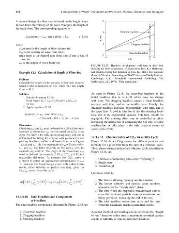
FIGURE 12.15 Headloss development with time in filter bed,
showing the three components. (Adapted from Ives, K.J. Mathemat-
Example 12.1 Calculation of Depth of Filter Bed ical models of deep bed filtration, in Ives, K.J. (Ed.), The Scientific
Basis of Filtration, Proceedings of NATO Advanced Study Institute,
Problem Cambridge, U.K., Noordhoff International Publishing, The
Calculate the length of filter column, L(filter bed), required Netherlands, 220, 1975c. With permission.)
based on the experiments of Ives (1962) for a run length,
t(run) ¼ 30 h.
Solution As seen in Figure 12.15, the clean-bed headloss is the
1. Data for Equation 12.10. initial headloss, that is, at t ¼ 0, which does not change
with time. The clogging headloss causes a linear headloss
From Figure 12.7, v wf ¼ 0.90 cm=h and L wf
16 cm. increase with time, and is the middle curve. Finally, the
2. Apply Equation 12.10, straining headloss increases exponentially with time, and is
the upper line. A goal in filtration is that the straining head-
L(column) v wf t(run time) þ L wf loss, due to its exponential increase with time, should be
¼ 0:90 cm=h 30 h þ 16 cm ¼ 43 cm negligible. The straining effect may be controlled by either
increasing the media size or decreasing the floc size, or some
Discussion combination. A pilot plant is the only practical means to
Obtaining v wf and L wf must be based on a pilot plant study. assess such effects.
Methods to determine v wf may be based on C(Z)t,oron
s(Z)t. The latter is the only practical approach and can be
determined by fitting the column with piezometers and 12.3.2.11 Characteristics of C(t) Z for a Filter Cycle
plotting headloss profiles at different times as in Figures Figure 12.16 shows C(t) Z curves for effluent particles and
12.13a and 12.16b. The magnitude of v wf will vary with v, turbidity for a pilot filter from the start of a filtration cycle.
C o and s u ; the latter depends on the media size, for Three phases characteristic of any filtration cycle, identified in
example, d 10 and UF. The length of the wave front, L wf , Figure 12.16, are
must be defined, for example, 0.05 C=C o 0.95, is a
reasonable definition. To measure the C(Z) t curve is
1. Chemical conditioning (also called ‘‘ripening’’)
a means to obtain an approximate determination of L wf .
To measure the breakthrough curve with online instru- 2. Steady state
ments, either turbidity or particle counting, gives the 3. Breakthrough
curve. From this curve
C(t) Z¼Z o
Questions relate to

C C 1. The factors affecting ripening and its duration.
0:95 :
Dt 0:05 0:95 v wf L wf 0:05
C o C o 2. The lowest turbidity and particle count numbers
attainable for the ‘‘steady state’’ phase.
3. The time when the respective breakthrough curves
cross the maximum particle count or maximum tur-
12.3.2.10 Total Headloss and Components
bidity permitted, indicating the end of the run.
of Headloss 4. The total headloss versus time curve and the time
The three headloss components, illustrated in Figure 12.15, are when the maximum headloss permitted occurs.
1. Clean-bed headloss As noted, the third and fourth questions determine the ‘‘length
2. Clogging headloss of run,’’ based on either time to maximum permitted particle
3. Straining headloss counts or turbidity or time to maximum headloss.