Page 235 - gas transport in porous media

Chapter 13: Lattice Boltzmann Method
30
0.8p 231
25
0.6p
20
1.0p
15
vU x /A 10 0.4p

5
1.2p
0
0.2p
–5
–10
0 0.2 0.4 0.6 0.8 1
r / R
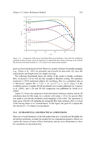
Figure 13.7. Comparison of theoretical normalized flow speed (unbroken lines) with LB calculations
(symbols) at different times (where the fractions of π indicate the time offsets in fractions of one period).
The abscissa is the radial position, R = 25 lu, and A is the axial pressure gradient

gases in closest-packed porous beds. However, models of deeper barometric pumping
(e.g., Nilson et al., 1991) are generally out-of-reach for pore-scale LB, since the
required time and length-scales are simply too large.
The following benchmark shows the ability of the model to handle oscillatory
flow; in Section 13.4 we will use this example to illustrate scaling. We reproduce
Lambossy’s (1952) analytical solution for oscillatory flow in a cylindrical tube at
a “Womersly” number Wo = 7.237 = R · (ω/ν) 1/2 , ω = 2π/T, where T is the
oscillation period. A similar 2D LB benchmark was recently published by Cosgrove
et al. (2003), and a 2D and 3D LB comparison was published by Artoli et al.
(2002).
Figure 13.7 shows the comparison of the theoretical Lambossy solution, and an LB
calculation done for this study, for a cylinder with radius = 25 lu. No special effort
was made to prevent the pixelation (stair-stepping) of the walls. The agreement is
quite good, with the LB capturing the antegrade flow that continues after a reversal
of the forcing (there is no “normalization” in this figure; the good fit is despite the
fact that the R = 25 channel was pixelated).

13.4 FUNDAMENTALAND PRACTICAL LIMITATIONS
There are several limitations of the LB method that give it insufficient flexibility for
all arbitrary problems, or make the method far too computation-intensive. Below we
explore the sources of some of these limitations, and use some illustrations to show
the constraints on calculation time.