Page 232 - gas transport in porous media

Stockman
228
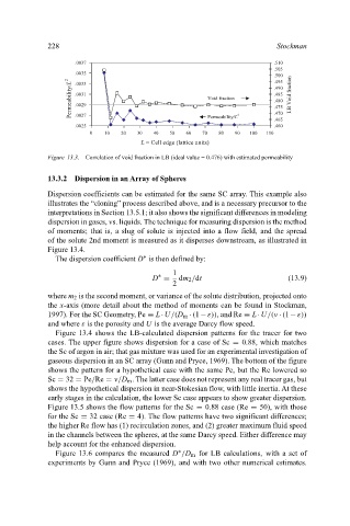
.510
.0037
.505
.0035 .500
Permeability/L 2 .0031 Void fraction .490 LB Void fraction
.495
.0033
.485
.480
.0029
.475
.470
2
.0027
Permeability/L
.465
.0025 .460
0 10 20 30 40 50 60 70 80 90 100 110
L = Cell edge (lattice units)
Figure 13.3. Correlation of void fraction in LB (ideal value = 0.476) with estimated permeability
13.3.2 Dispersion in an Array of Spheres
Dispersion coefficients can be estimated for the same SC array. This example also
illustrates the “cloning” process described above, and is a necessary precursor to the
interpretations in Section 13.5.1; it also shows the significant differences in modeling
dispersion in gases, vs. liquids. The technique for measuring dispersion is the method
of moments; that is, a slug of solute is injected into a flow field, and the spread
of the solute 2nd moment is measured as it disperses downstream, as illustrated in
Figure 13.4.
∗
The dispersion coefficient D is then defined by:
1
∗
D = dm 2 /dt (13.9)
2
where m 2 is the second moment, or variance of the solute distribution, projected onto
the x-axis (more detail about the method of moments can be found in Stockman,
1997). For the SC Geometry, Pe ≡ L·U/(D m ·(1−ε)), and Re ≡ L·U/(ν ·(1−ε))
and where ε is the porosity and U is the average Darcy flow speed.
Figure 13.4 shows the LB-calculated dispersion patterns for the tracer for two
cases. The upper figure shows dispersion for a case of Sc = 0.88, which matches
the Sc of argon in air; that gas mixture was used for an experimental investigation of
gaseous dispersion in an SC array (Gunn and Pryce, 1969). The bottom of the figure
shows the pattern for a hypothetical case with the same Pe, but the Re lowered so
Sc = 32 = Pe/Re = ν/D m . The latter case does not represent any real tracer gas, but
shows the hypothetical dispersion in near-Stokesian flow, with little inertia. At these
early stages in the calculation, the lower Sc case appears to show greater dispersion.
Figure 13.5 shows the flow patterns for the Sc = 0.88 case (Re = 50), with those
for the Sc = 32 case (Re = 4). The flow patterns have two significant differences;
the higher Re flow has (1) recirculation zones, and (2) greater maximum fluid speed
in the channels between the spheres, at the same Darcy speed. Either difference may
help account for the enhanced dispersion.
∗
Figure 13.6 compares the measured D /D m for LB calculations, with a set of
experiments by Gunn and Pryce (1969), and with two other numerical estimates.