Page 172 - Geochemical Anomaly and Mineral Prospectivity Mapping in GIS

Analysis of Geologic Controls on Mineral Occurrence 173

usually not Poisson-distributed. Secondly, the distance distribution method assumes that
the linear (or point) geological features under examination have both uniform and
random distribution in a study area (Berman, 1977). Certainly, in many cases, this
assumption is inapplicable; linear (or point) geological features may exhibit clustering in
some parts of a study area and/or are sparse in other parts of a study area. Anyhow, the
problem associated with this assumption about the distribution of linear (or point)
geological features is avoided by using either a very large number of uniformly
distributed random points (Bonham-Carter, 1985; Berman, 1986) or all pixels in a study
area (Bonham-Carter, 1994). Finally, one wonders why all lines in a set of lines (e.g., all
NNW-trending faults) are used in the analysis even if mineral deposits are associated
with only some of these lines. The following section explains another method, in which
only lines (or points) nearest to points of interests are used in the spatial association
analysis.

Distance correlation method
The concept of the distance correlation method was developed and demonstrated by
Carranza (2002) and Carranza and Hale (2002b) to characterise quantitatively spatial
association between a set of points of interest (i.e., occurrences of mineral deposits of the
type sought and a set of lines (e.g., faults/fractures) or points (e.g., centroids of porphyry
stocks). This method is a non-parametric test of spatial association between a set of point
geo-objects and a set of linear (or point) geo-objects because it does not involve testing
statistical significance of spatial association. However, as demonstrated by Carranza
(2002) and Carranza and Hale (2002b) and by the results of analyses in this volume, the
method provides results that are similar to the results obtained by application of the
distance distribution method.
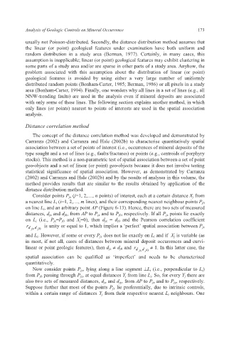
Consider points P jx (j=1, 2,…, n points) of interest, each at a certain distance X j from
a nearest line L i (i=1, 2,…, m lines), and their corresponding nearest neighbour points P j0
on line L i, and an arbitrary point AP (Figure 6-13). Hence, there are two sets of measured
distances, d jx and d j0, from AP to P jx and to P j0, respectively. If all P jx points lie exactly
on L i (i.e., P jx=P j0 and X j=0), then d jx = d j0 and the Pearson correlation coefficient
r d jx d 0 j is unity or equal to 1, which implies a ‘perfect’ spatial association between P jx
and L i. However, if some or every P jx does not lie exactly on L i and if X j is variable (as
in most, if not all, cases of distances between mineral deposit occurrences and curvi-
linear or point geologic features), then d jx ≠ d j0 and r d jx d 0 j ≠ 1. In this latter case, the
spatial association can be qualified as ‘imperfect’ and needs to be characterised
quantitatively.
Now consider points P jy, lying along a line segment ⊥L i (i.e., perpendicular to L i)
from P j0 passing through P jx, at equal distances Y j from line L i. So, for every Y j there are
also two sets of measured distances, d jx and d jy , from AP to P jx and to P jy, respectively.
Suppose further that most of the points P jx lie preferentially, due to intrinsic controls,
within a certain range of distances Y j from their respective nearest L i neighbours. One