Page 262 - Geochemical Anomaly and Mineral Prospectivity Mapping in GIS
P. 262
Data-Driven Modeling of Mineral Prospectivity                        265

           every deposit-type, proxy deposit-type and non-deposit location. By  modeling a
           mathematical relationship between a set of mineral occurrence scores (Y i) and multiple
           sets of  MOFS ji of spatial data at deposit-type, proxy deposit-type and  non-deposit
           locations, weak dissimilarities in multivariate spatial data signatures  of  deposit-type
           locations and weak to moderate dissimilarities in multivariate spatial data signatures of
           proxy deposit-type locations, as indicated in Fig. 8-6, can be enhanced. This allows
           distinction between coherent and  non-coherent  deposit-type locations and  between
           coherent  and non-coherent proxy  deposit-type locations. Then a threshold  Ǔ i can  be
           sought to distinguish between coherent and  non-coherent deposit-type locations and
           between coherent and non-coherent proxy deposit-type locations.
              Because the  mineral occurrence score,  Y i, is a dichotomous  variable, logistic
           regression is appropriate in modeling the relationship between Y i and MOFS ji in order to
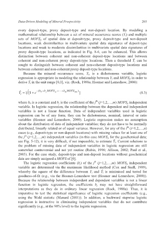
           derive Ǔ i in the unit range [0,1], viz. (Rock, 1988a; Hosmer and Lemeshow, 2000):

            ˆ
           Y = 1  1 [ +  e − (b + b j MOFS +" + b m MOFS mn ) ]                (8.3)
                        0
                                ji
            i

                                                      th
           where b 0 is a constant and b j is the coefficient of the j  (j=1,2,…,m) MOFS ji independent
           variable. In logistic regression, the relationship between the dependent and independent
           variables is  not a linear  function.  Data  of independent variables  used in logistic
           regression  can  be of any form;  they  can be  dichotomous,  nominal, interval or ratio
           variables (Hosmer and Lemeshow,  2000). Logistic regression makes no assumption
           about the distribution of data of independent variables; they do not have to be normally
                                                                        th
           distributed, linearly related or of equal variance. However, for any of the i  (i=1,2,…,n)
           cases (e.g., deposit-type or non-deposit locations) with missing values for at least one of
               th
           the j  (j=1,2,…,m) independent variables (in this case MOFS ji for the geochemical data;
           see Fig. 5-12), it is very difficult, if not impossible, to estimate Ǔ i. Current solutions to
           the problem of missing data of independent variables in logistic regression are still
           somewhat controversial and  not yet routine (Rubin, 1996; Allison,  2002; Paul et al.,
           2003). For the case study, deposit-type and non-deposit locations without geochemical
           data are simply assigned a MOFS of [0].
                                                     th
              The logistic regression coefficients (b j) of the j  (j=1,2,…,m) MOFS ji independent
           variable are determined via  the maximum likelihood method (Cox and Snell,  1989),
           whereby the  square  of the difference  between  Y i and  Ǔ i  is minimised and tested for
           goodness-of-fit (e.g., via the Hosmer-Lemeshow test (Hosmer and Lemeshow, 2000)).
           Because the relationship between independent and dependent variables is not a linear
           function in logistic  regression, the coefficients  b j may not have  straightforward
           interpretations as they do in ordinary linear regression (Rock, 1988a). Thus, it is
           imperative to test the statistical significance  of logistic regression coefficients (e.g.,
           using the  Wald statistic (Menard (2001)). In addition,  a backward stepwise logistic
           regression is instructive in eliminating independent variables that do not contribute
           significantly (e.g., at the 90% level) to the logistic regression.

