Page 293 - Geochemical Anomaly and Mineral Prospectivity Mapping in GIS

296 Chapter 8

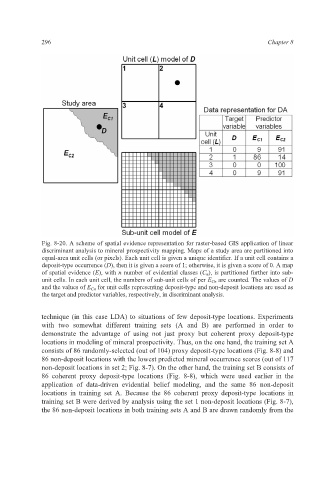
Fig. 8-20. A scheme of spatial evidence representation for raster-based GIS application of linear
discriminant analysis to mineral prospectivity mapping. Maps of a study area are partitioned into
equal-area unit cells (or pixels). Each unit cell is given a unique identifier. If a unit cell contains a
deposit-type occurrence (D), then it is given a score of 1; otherwise, it is given a score of 0. A map
of spatial evidence (E), with n number of evidential classes (C n ), is partitioned further into sub-
unit cells. In each unit cell, the numbers of sub-unit cells of per E Cn are counted. The values of D
and the values of E Cn for unit cells representing deposit-type and non-deposit locations are used as
the target and predictor variables, respectively, in discriminant analysis.

technique (in this case LDA) to situations of few deposit-type locations. Experiments
with two somewhat different training sets (A and B) are performed in order to
demonstrate the advantage of using not just proxy but coherent proxy deposit-type
locations in modeling of mineral prospectivity. Thus, on the one hand, the training set A
consists of 86 randomly-selected (out of 104) proxy deposit-type locations (Fig. 8-8) and
86 non-deposit locations with the lowest predicted mineral occurrence scores (out of 117
non-deposit locations in set 2; Fig. 8-7). On the other hand, the training set B consists of
86 coherent proxy deposit-type locations (Fig. 8-8), which were used earlier in the
application of data-driven evidential belief modeling, and the same 86 non-deposit
locations in training set A. Because the 86 coherent proxy deposit-type locations in
training set B were derived by analysis using the set 1 non-deposit locations (Fig. 8-7),
the 86 non-deposit locations in both training sets A and B are drawn randomly from the