Page 290 - Geochemical Anomaly and Mineral Prospectivity Mapping in GIS

Data-Driven Modeling of Mineral Prospectivity 293

DISCRIMINANT ANALYSIS OF MINERAL PROSPECTIVITY
Discriminant analysis (DA) has a long history of application in exploration
geochemistry (e.g., Bull and Mazzucchelli, 1975; Govett et al., 1975; Beauchamp et al.,
1980; Howarth, 1983b; Clarke et al., 1989; Chork and Rousseeuw, 1992; Yusta et al.,
1998; Singer and Kouda, 2001) and mineral prospectivity mapping (see references in
Table 8-II). The common chief objective of the applications of DA to geochemical
anomaly and mineral prospectivity mapping is to classify every location in a study area
into two mutually exclusive groups – prospective (anomalous or mineralised) and non-
prospective (background or barren) – based on a training set of known deposit-type and
non-deposit locations and multiple sets of data of discriminating (i.e.,
predictor/explanatory) variables at these locations.
Exhaustive explanations of DA are not given here, but readers are referred to Davis
(2002, pp. 471-479) for a thorough introduction to DA and to Harris and Pan (1999) and
Pan and Harris (2000, pp.411-414) for explanations of different methods of DA that can
be applied to mineral prospectivity modeling. The treatment of DA here is limited to the
basic principles and application of the two-group DA method, which is also called Fisher
linear DA (Fisher, 1936) and demonstration of a GIS-based technique for representation
of data of predictor/explanatory variables in DA.

Basic principles and assumptions of linear discriminant analysis
In general, the maximum number of discriminant functions that can be derived for
the classification of groups of data is either equal to the number of groups minus one or
equal to the number of predictor variables, whichever is less. In the two-group DA
(hereafter denoted as LDA; L stands for linear), therefore, there is only one discriminant
function, which is a linear combination of the predictor variables with the following
mathematical form:

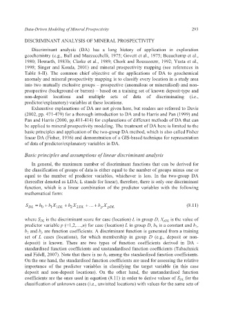
S DL = b + b 1 X 1 DL + b 2 X 2 DL +! + b p X pDL (8.11)
0

where S DL is the discriminant score for case (location) L in group D, X pDL is the value of
predictor variable p (=1,2,…,n) for case (location) L in group D, b 0 is a constant and b 1,
b 2 and b p are function coefficients. A discriminant function is generated from a training
set of L cases (locations), for which membership in group D (e.g., deposit or non-
deposit) is known. There are two types of function coefficients derived in DA -
standardised function coefficients and unstandardised function coefficients (Tabachnick
and Fidell, 2007). Note that there is no b 0 among the standardised function coefficients.
On the one hand, the standardised function coefficients are used for assessing the relative
importance of the predictor variables in classifying the target variable (in this case
deposit and non-deposit locations). On the other hand, the unstandardised function
coefficients are the ones used in equation (8.11) in order to derive values of S DL for the
classification of unknown cases (i.e., unvisited locations) with values for the same sets of