Page 115 - Geothermal Energy Renewable Energy and The Environment

Exploring for Geothermal Systems 101

400

350
Computed SiO 2 temperature (°C) 250
300

200

150

100

50
0
0 50 100 150 200 250 300 350 400
Computed Na–K temperature (°C)

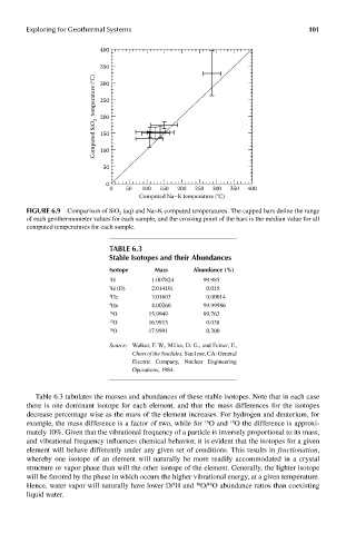
FIGUre 6.9 Comparison of SiO 2 (aq) and Na–K computed temperatures. The capped bars define the range
of each geothermometer values for each sample, and the crossing point of the bars is the median value for all
computed temperatures for each sample.

Table 6.3
stable Isotopes and their abundances
Isotope mass abundance (%)
1 H 1.007824 99.985
2 H (D) 2.014101 0.015
3 He 3.01603 0.00014
4 He 4.00260 99.99986
16 O 15.9949 99.762
17 O 16.9913 0.038
18 O 17.9991 0.200

Source: Walker, F. W., Miller, D. G., and Feiner, F.,
Chart of the Nuclides, San Jose, CA: General
Electric Company, Nuclear Engineering
Operations, 1984.

Table 6.3 tabulates the masses and abundances of these stable isotopes. Note that in each case
there is one dominant isotope for each element, and that the mass differences for the isotopes
decrease percentage wise as the mass of the element increases. For hydrogen and deuterium, for
16
example, the mass difference is a factor of two, while for O and O the difference is approxi-
18
mately 10%. Given that the vibrational frequency of a particle is inversely proportional to its mass,
and vibrational frequency influences chemical behavior, it is evident that the isotopes for a given
element will behave differently under any given set of conditions. This results in fractionation,
whereby one isotope of an element will naturally be more readily accommodated in a crystal
structure or vapor phase than will the other isotope of the element. Generally, the lighter isotope
will be favored by the phase in which occurs the higher vibrational energy, at a given temperature.
16
Hence, water vapor will naturally have lower D/ H and O/ O abundance ratios than coexisting
1
18
liquid water.