Page 171 - Geothermal Energy Renewable Energy and The Environment

Generating Power Using Geothermal Resources 157

1000.0

100.0 300°C
Liquid 250°C
1
200°C Vapor
10.0 150°C
Pressure (bars) 1.0 100°C

0.1 50°C
2 2 *
25°C
0.01
Liquid + Vapor
0.001
0.0 2.0 4.0 6.0 8.0 10.0
Entropy (kJ/kg)

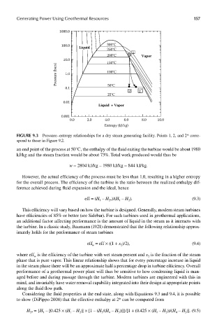
FIGUre 9.3 Pressure–entropy relationships for a dry steam generating facility. Points 1, 2, and 2* corre-
spond to those in Figure 9.2.
an end point of the process at 50°C, the enthalpy of the fluid exiting the turbine would be about 1980
kJ/kg and the steam fraction would be about 73%. Total work produced would thus be

w = 2804 kJ/kg – 1980 kJ/kg = 844 kJ/kg.

However, the actual efficiency of the process must be less than 1.0, resulting in a higher entropy
for the overall process. The efficiency of the turbine is the ratio between the realized enthalpy dif-
ference achieved during fluid expansion and the ideal, hence
eff = (H – H )/(H – H ). (9.3)
2*
1
2
1
This efficiency will vary based on how the turbine is designed. Generally, modern steam turbines
have efficiencies of 85% or better (see Sidebar). For such turbines used in geothermal applications,
an additional factor affecting performance is the amount of liquid in the steam as it interacts with
the turbine. In a classic study, Baumann (1921) demonstrated that the following relationship approx-
imately holds for the performance of steam turbines
eff = eff × ((1 + x )/2), (9.4)
2
w
where eff is the efficiency of the turbine with wet steam present and x is the fraction of the steam
2
w
phase that is pure vapor. This linear relationship shows that for every percentage increase in liquid
in the steam phase there will be an approximate half a percentage drop in turbine efficiency. Overall
performance of a geothermal power plant will thus be sensitive to how condensing liquid is man-
aged before and during passage through the turbine. Modern turbines are engineered with this in
mind, and invariably have water removal capability integrated into their design at appropriate points
along the fluid flow path.
Considering the fluid properties at the end state, along with Equations 9.3 and 9.4, it is possible
to show (DiPippo 2008) that the effective enthalpy at 2* can be computed from
H = {H – [0.425 × (H – H )] × [1 – (H /(H – H ))]}/[1 + (0.425 × (H – H ))/(H – H )]. (9.5)
4
2
3
1
1
1
2*
2
3
4
3