Page 220 - Glucose Monitoring Devices

The retrofitting algorithm 223

Step A: Retrospective Baysian CGM Recalibration
450
(Input) Outlier−checked CGM
400 (Input) Outlier−checked BG References
(Input) Calibrations
Concentration [mg/dl] 300
350
(Output) Recalibrated CGM
Test BG Reference
250
200
150
100
50
18:00 00:00 06:00 12:00 18:00
Time [hh:mm]
Step B: Constrained Regularized Deconvolution
450
(Input) Recalibrated CGM
400 (Input) Oulier−checked BG References
(Output) Retrofitted BG
Concentration [mg/dl] 300
350
Test BG Reference
CGM
250
200
150
100
50
18:00 00:00 06:00 12:00 18:00
Time [hh:mm]
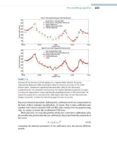
FIGURE 11.2
Example of the two-step method applied on a representative dataset. Top panel:
retrospective Bayesian CGM recalibration (Step A) enhances accuracy of the CGM.
Bottom panel: constrained regularized deconvolution (Step B) simultaneously
compensates for the distortion introduced by the blood-to-interstitium glucose transport
and reduces measurement noise exploiting the physiological prior on BG smoothness. To
assess the quality of the reconstruction, both panels also show the test BG references
(empty diamonds), to which the retrofitting algorithm had no access.

Bayesian estimation procedure. Subsequently, calibration errors are compensated on
the basis of these estimates (recalibration). As inputs, Step A takes calibration data
together with outliers-checked CGM and BGs data coming from the preprocessing
step. As output, it returns the recalibrated CGM trace.
More precisely, for each data portion among two consecutive calibrations (plus
the possible data portion after the last calibration), Step A performs the estimation of
the vector
T
q ¼½a; b; g; sŠ (11.6)
containing the unknown parameters of the calibration error and glucose diffusion
models.