Page 221 - Glucose Monitoring Devices

224 CHAPTER 11 Retrofitting CGM traces

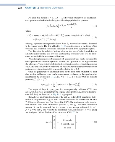
For each data portion k ¼ 1; .; K þ 1, a Bayesian estimate of the calibration-
error parameters is obtained solving the following optimization problem:

h i
argminJðqÞ
b b (11.7)
k k
b a k ; b ; b g ; b s k ¼ q k ¼
q
where
T 1
k k
JðqÞ¼ðcgm k aig ðsÞ b gDt k Þ S w k :ðcgm k aig ðsÞ b gDt k Þ
(11.8)
X 1
T
þðq m Þ ðq m Þ
q q
q
where m represents the expected value of q and S q its covariance matrix, discussed
q
in the remark below. The first addend in (11.8) penalizes errors in the fitting of the
observed data while the second one penalizes deviation from a population prior.
This Bayesian formulation, besides allowing the use of prior knowledge on
calibration-error model, also prevents identifiability problems when few BG refer-
ences are available between two calibrations.
When the optimization problem is solved, a number of tests can be performed to
detect presence of abnormal dynamics in the CGM signal that do not appear also in
the references. These tests include the final cost function value, estimated parameter
value, and their coefficient-of-variation. An effective rule of thumb is to exclude data
portion where the estimated b a k was smaller, that is, b a k < 0:3.
Once the parameters of calibration-error model have been estimated for each
data portion, calibration error can be compensated performing a data-portion-wise
recalibration by inversion of (11.2), i.e., ck ¼ 1; .; K þ 1 and ct in the kth data
cal
portion (t cal t < t ):
k 1 k
1 cal
cgmðtÞ b b g t t : (11.9)
b
cgm recal ðtÞ¼ k 1
b a k
The output of Step A, cgm recal ðtÞ, is a retrospectively calibrated CGM time
series, which is more accurate than the original CGM profile (i.e., closer to the refer-
ence BG data), as illustrated in Fig. 11.2, upper panel.
Remark: Let us discuss the choice of S q and m .InRef.[16], population distri-
q
bution of the parameters a; b; g, and s has been estimated for the Dexcom SEVEN
PLUS sensor (Dexcom Inc., San Diego, CA, USA). The joint second-order descrip-
tion obtained from these distribution provides S q and m . For other commercial
q
sensors, it can be assumed that the sensor is on average calibrated (a ¼ 1,
b ¼ g ¼ 0) and s q can be set to the population value, for instance, s q ¼ 15 [min]
for Navigator (Abbott Diabetes Care, Alameda, CA) [17], i.e.,
2 3 2 3
1
a
6 7 6 7
6 7 6 7
b 0 ½mg=dLŠ
6 7 6 7
m ¼ E6 7 ¼ 6 7: (11.10)
q
6 7 6 7
g 0 ½mg=dL=minŠ
4 5 4 5
s 15 ½minŠ