Page 223 - Glucose Monitoring Devices

226 CHAPTER 11 Retrofitting CGM traces

where C is the m M selection matrix obtained removing from the M M identity
matrix all the rows except the t 1 ; .; t m -th ones, i.e., all the entries of C are zeros,
except for the ones in position ði; t i Þ, equal to 1. Although BG references are highly
accurate there is always a confidence interval around the measurement where the
true concentration can lay, so that the above Eq. (11.13) becomes
r
l ci ðbgÞ C$bg u ci ðbgÞ (11.15)
where l ci ðbgÞ$(u ci ðbgÞ) is the ℝ m vectors of lower (upper) limits delimiting
measurements Confidence Intervals and the inequality is meant element-wise. As
an example, YSI is guaranteed to introduce an error of at most 2%, therefore
(11.14) reduces to
r
0:98 $ bg C$bg 1:02$bg (11.16)
Note that (11.14) easily allows addressing of different accuracies of different
reference measurement instruments such as YSI, Hemocue, or traditional capillary
finger prick measurements (SMBG). Moreover, it allows taking into account
different accuracies of the same instruments in different measurement regions.
The constraint expressed in Eq. (11.14) will be explicitly taken into account in
the estimation of the blood glucose concentration with a constrained regularized
deconvolution in the form of a constrained Tikhonov regularization problem.
To perform the deconvolution in the classical linear time-invariant system frame-
work, s in (11.1) is fixed to the average of the s i previously estimated for each data
portion:
Kþ1
1 X
b s k (11.17)
K þ 1
s ¼
k¼1
Then it holds
r
cgm recal ðtÞ¼ G$bg þ w recal ; (11.18)
where G is the n M rectangular submatrix of the M M transfer matrix G M M ðsÞ,
cgm cgm
obtained retaining only the t ; .; t n th columns of G M M ðsÞ. The noise w recal
1
description can be obtained by noting that, from (11.8), it follows
1
w recal ðtÞ¼ wðtÞ, so that the covariance matrix of w recal can be well approximated
^ a k
with a block diagonal matrix,
!
1 1
S ¼ BlockDiag S w ; .; S w : (11.19)
2 2
b a 1 b a Kþ1
To formulate the constrained Tikhonov regularization problem, let us introduce
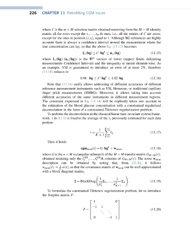
the Toeplitz matrix F:
2 3
1 0
1 1
6 7
6 7
F ¼ 6 7 (11.20)
4 1 1 5
0 1 1