Page 218 - Glucose Monitoring Devices

The retrofitting algorithm 221

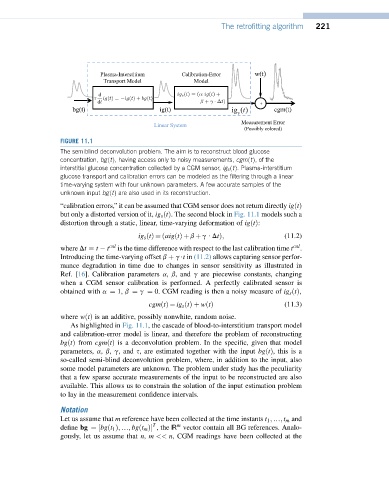
FIGURE 11.1
The semiblind deconvolution problem. The aim is to reconstruct blood glucose
concentration, bgðtÞ, having access only to noisy measurements, cgmðtÞ, of the
interstitial glucose concentration collected by a CGM sensor, ig s ðtÞ. Plasma-interstitium
glucose transport and calibration errors can be modeled as the filtering through a linear
time-varying system with four unknown parameters. A few accurate samples of the
unknown input bgðtÞ are also used in its reconstruction.

“calibration errors,” it can be assumed that CGM sensor does not return directly igðtÞ
but only a distorted version of it, ig s ðtÞ. The second block in Fig. 11.1 models such a
distortion through a static, linear, time-varying deformation of igðtÞ:
ig s ðtÞ¼ðaigðtÞþ b þ g $ DtÞ; (11.2)
cal
where Dt ¼ t t cal is the time difference with respect to the last calibration time t .
Introducing the time-varying offset b þ g$t in (11.2) allows capturing sensor perfor-
mance degradation in time due to changes in sensor sensitivity as illustrated in
Ref. [16]. Calibration parameters a, b, and g are piecewise constants, changing
when a CGM sensor calibration is performed. A perfectly calibrated sensor is
obtained with a ¼ 1, b ¼ g ¼ 0. CGM reading is then a noisy measure of ig s ðtÞ,
(11.3)
cgmðtÞ¼ ig s ðtÞþ wðtÞ
where wðtÞ is an additive, possibly nonwhite, random noise.
As highlighted in Fig. 11.1, the cascade of blood-to-interstitium transport model
and calibration-error model is linear, and therefore the problem of reconstructing
bgðtÞ from cgmðtÞ is a deconvolution problem. In the specific, given that model
parameters, a, b, g, and s, are estimated together with the input bgðtÞ, this is a
so-called semi-blind deconvolution problem, where, in addition to the input, also
some model parameters are unknown. The problem under study has the peculiarity
that a few sparse accurate measurements of the input to be reconstructed are also
available. This allows us to constrain the solution of the input estimation problem
to lay in the measurement confidence intervals.
Notation
Let us assume that m reference have been collected at the time instants t 1 ; .; t m and
m
T
define bg ¼½bgðt 1 Þ; .; bgðt m ފ , the ℝ vector contain all BG references. Analo-
gously, let us assume that n, m << n, CGM readings have been collected at the