Page 219 - Glucose Monitoring Devices

222 CHAPTER 11 Retrofitting CGM traces

cgm cgm cgm cgm T
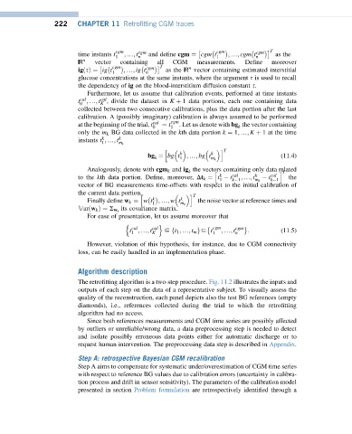
time instants t 1 ; .; t n and define cgm ¼ cgm t 1 ; .; cgm t n as the
ℝ n vector containing all CGM measurements. Define moreover
cgm T n
igðsÞ¼ ig t ; .; ig t cgm as the ℝ vector containing estimated interstitial
1 n
glucose concentrations at the same instants, where the argument s is used to recall
the dependency of ig on the blood-interstitium diffusion constant s.
Furthermore, let us assume that calibration events, performed at time instants
cal
cal
t ; .; t , divide the dataset in K þ 1 data portions, each one containing data
0 K
collected between two consecutive calibrations, plus the data portion after the last
calibration. A (possibly imaginary) calibration is always assumed to be performed
at the beginning of the trial, t cal ¼ t cgm . Let us denote with bg the vector containing
0 1 k
only the m k BG data collected in the kth data portion k ¼ 1; .; K þ 1 at the time
k
instants t ; .; t k
1 m k
h i T
k k
bg ¼ bg t 1 ; .; bg t m k (11.4)
k
Analogously, denote with cgm k and ig the vectors containing only data related
k
T
h
i
cal
k
k
to the kth data portion. Define, moreover, Dt k ¼ t t k 1 ; .; t m k t cal the
k 1
1
vector of BG measurements time-offsets with respect to the initial calibration of
the current data portion. h i T

k
Finally define w k ¼ w t ; .; w t k the noise vector at reference times and
1 m k
its covariance matrix.
Varðw k Þ¼ S w k
For ease of presentation, let us assume moreover that
n o cgm
cal
t ; .; t cal 4 ft 1 ; .; t m g4 t ; .; t cgm : (11.5)
1 K 1 n
However, violation of this hypothesis, for instance, due to CGM connectivity
loss, can be easily handled in an implementation phase.
Algorithm description
The retrofitting algorithm is a two-step procedure. Fig. 11.2 illustrates the inputs and
outputs of each step on the data of a representative subject. To visually assess the
quality of the reconstruction, each panel depicts also the test BG references (empty
diamonds), i.e., references collected during the trial to which the retrofitting
algorithm had no access.
Since both references measurements and CGM time series are possibly affected
by outliers or unreliable/wrong data, a data preprocessing step is needed to detect
and isolate possibly erroneous data points either for automatic discharge or to
request human intervention. The preprocessing data step is described in Appendix.
Step A: retrospective Bayesian CGM recalibration
Step A aims to compensate for systematic under/overestimation of CGM time series
with respect to reference BG values due to calibration errors (uncertainty in calibra-
tion process and drift in sensor sensitivity). The parameters of the calibration model
presented in section Problem formulation are retrospectively identified through a