Page 246 - How To Implement Lean Manufacturing

224 Cha pte r F i f tee n

Cell 2 Time Study
35
30
25
Time (secs) 20 Their Study

15
Our Study
10
5
0
1 2 3 4 5
Work station
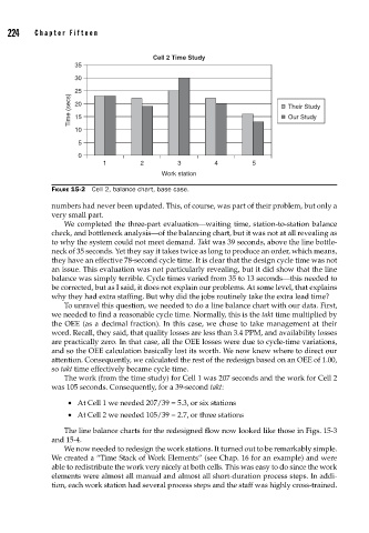
FIGURE 15-2 Cell 2, balance chart, base case.

numbers had never been updated. This, of course, was part of their problem, but only a
very small part.
We completed the three-part evaluation—waiting time, station-to-station balance
check, and bottleneck analysis—of the balancing chart, but it was not at all revealing as
to why the system could not meet demand. Takt was 39 seconds, above the line bottle-
neck of 35 seconds. Yet they say it takes twice as long to produce an order, which means,
they have an effective 78-second cycle time. It is clear that the design cycle time was not
an issue. This evaluation was not particularly revealing, but it did show that the line
balance was simply terrible. Cycle times varied from 35 to 13 seconds—this needed to
be corrected, but as I said, it does not explain our problems. At some level, that explains
why they had extra staffing. But why did the jobs routinely take the extra lead time?
To unravel this question, we needed to do a line balance chart with our data. First,
we needed to find a reasonable cycle time. Normally, this is the takt time multiplied by
the OEE (as a decimal fraction). In this case, we chose to take management at their
word. Recall, they said, that quality losses are less than 3.4 PPM, and availability losses
are practically zero. In that case, all the OEE losses were due to cycle-time variations,
and so the OEE calculation basically lost its worth. We now knew where to direct our
attention. Consequently, we calculated the rest of the redesign based on an OEE of 1.00,
so takt time effectively became cycle time.
The work (from the time study) for Cell 1 was 207 seconds and the work for Cell 2
was 105 seconds. Consequently, for a 39-second takt:
• At Cell 1 we needed 207/39 = 5.3, or six stations
• At Cell 2 we needed 105/39 = 2.7, or three stations
The line balance charts for the redesigned flow now looked like those in Figs. 15-3
and 15-4.
We now needed to redesign the work stations. It turned out to be remarkably simple.
We created a “Time Stack of Work Elements” (see Chap. 16 for an example) and were
able to redistribute the work very nicely at both cells. This was easy to do since the work
elements were almost all manual and almost all short-duration process steps. In addi-
tion, each work station had several process steps and the staff was highly cross-trained.