Page 192 - Hybrid-Renewable Energy Systems in Microgrids

Sensitivity and transient stability analysis of fixed speed wind generator 173

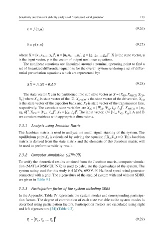
x = ( f xu, ) (9.26) x˙=fx,u

0 = ( gx, ) u (9.27) 0=gx,u

T
T
where X = [x 1 ,x 2 ,….x n ] , u = [u 1 ,u 2 ,….u n ], g = [g 1 ,g 2 ,….g m ] . X is the state vector, u
is the input vector, g is the vector of output nonlinear equations.
The nonlinear equations are linearized around a nominal operating point to find a
set of linearized differential equations for the overall system rendering a set of differ-
ential perturbation equations which are represented by:

•
∆ X = A X∆+ B U (9.28) ∆X•=A.∆X+B.∆U
∆
.
.
The state vector X can be partitioned into sub state vector as X = [X , X MECH X ,
CB
IG
X ] where X is state vector of the IG, X MECH is the state vector of the drive train, X
T
IG
CB
is the state vector of the capacitor bank and X is state vector of the transmission line,
T
T
respectively. The associate state variables are X = [Ψ , Ψ , I , I ] , X MECH = [w ,
rd
sq
t
rq
IG
sd
T
T
T
w , θ] , X = [V , V ] , X = [I , I ] . The input vector, U= [V , V , V ]. A and B
CB
T
dg
sq
w
qt
dt
sd
r
qg
are constant matrices with appropriate dimensions.
2.3.1 Analysis using Jacobian Matrix
The Jacobian matrix is used to analyze the small signal stability of the system. The
equilibrium point X is calculated by solving the equation f(X ,U ) = 0. This Jacobian
o
o
o
matrix is derived from the state matrix and the elements of this Jacobian matrix will
be used to perform sensitivity result.
2.3.2 Computer simulation (LINMOD)
To verify the theoretical results obtained from the Jacobian matrix, computer simula-
tion (MATLAB/SIMULINK) is used to calculate the eigenvalues of the system. The
system rating used for this study is 4 MVA, 690 V, 60 Hz fixed speed wind generator
connected with a grid. The eigenvalues of the studied system with and without SDBR
are given in Table 9.1.
2.3.3 Participation factor of the system including SDBR
In the Appendix, Table IV represents the system modes and corresponding participa-
tion factors. The degree of contribution of each state variable to the system modes is
described using participation factors. Participation factors are calculated using right
and left eigenvectors [24] (Table 9.2).
P = [P ,P , …P ] T (9.29)
i 1i 2i ni
Pi=P1i, P2i,…PniT