Page 193 - Hybrid-Renewable Energy Systems in Microgrids

174 Hybrid-Renewable Energy Systems in Microgrids

∂ λ
Pki=∂λi∂αki=ψikφki P ki = i = ψφ ki (9.30)
ik
∂
α
ki
Ψ ik is the kth element of the ith left eigenvector of state matrix A, and Φ is the ith
ki
right eigenvector of state matrix A. The following observations are found from the
modal analysis of the studied system including SDBR:
1. Electrical Modes: The mode λ 1 ,λ 2 ,λ 3 , and λ 4 have the highest participation factors from state
variables V sd , V sq , I dt , and I dq .
2. Stator Mode: The modes λ 5 and λ 6 are associated with the state variables Ψ sd , Ψ sq , I dt , and
I qt . The network frequency is the corresponding frequency which is 60 Hz.
3. Electromechanical Mode: The modes λ 7 and λ 8 are associated with the state variables w r , θ,
and I rd . The corresponding natural frequency is 4.28 Hz.
4. Mechanical Mode: The modes λ 9 and λ 10 are associated with the state variables w t , θ, and I r .
The corresponding natural frequency is 0.62 Hz.
5. Monotonic Mode: The mode λ 11 is associated with the state variables Ψ sq and I rq .

2.4 Sensitivity analysis
Eigenvalue sensitivity is defined as the rate and direction of eigenvalue displacement in
the s-plane due to the variation in the system parameters. The first order sensitivity of an
eigenvalue λ i with regard to a system parameter α is given by the following equations:

∂λi∂α=φiT(∂A/∂α)ψiφiTψi ∂ λ φ ∂A( / ∂ α ψ )
T
i = i i (9.31)
∂ α φψ i
T
i
where Φ and Ψ are the right and left eigenvectors. Herein, the eigenvalues sensitiv-
i
i
ity with respect to drive train, generator, and transmission line parameters, with and
without SDBR are analyzed.
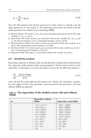
Table 9.1 The eigenvalues of the studied system with and without
SDBR

Eigenvalues (without
No. SDBR) Eigenvalues (with SDBR)

λ 1 −15.9 + j3111.3 −284.7 + j3880.7
λ 2 −15.9−j3111.3 −284.7−j3880.7
λ 3 −16.2 + j2355.7 −284.9 + j3126.5
λ 4 −16.2 - j2355.7 −284.9−j3126.5
λ 5 −15.7 + j376.8 −187.8 + j375.8
λ 6 −15.7−j376.8 −187.8 + j375.8
λ 7 −2.3 + j27.4 −0.9 + j27.9
λ 8 −2.3 − j27.4 −0.9−j27.9
λ 9 −0.3 + j4.2 −0.2 + j4.3
λ 10 −0.3 − j4.2 −0.2−j4.3
λ 11 −4.2 −4.1