Page 197 - Hydrocarbon Exploration and Production Second Edition

184 Expressing Uncertainty

7.2.3. Generating expectation curves
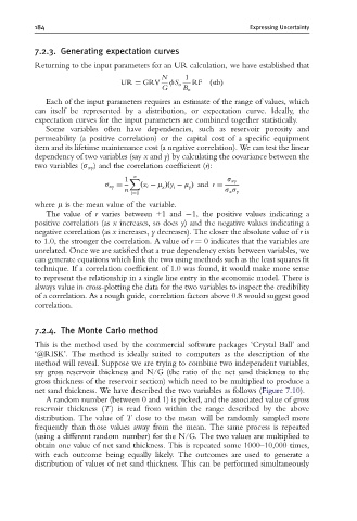
Returning to the input parameters for an UR calculation, we have established that
N 1
UR ¼ GRV fS o RF ðstbÞ
G B o
Each of the input parameters requires an estimate of the range of values, which
can itself be represented by a distribution, or expectation curve. Ideally, the
expectation curves for the input parameters are combined together statistically.
Some variables often have dependencies, such as reservoir porosity and
permeability (a positive correlation) or the capital cost of a specific equipment
item and its lifetime maintenance cost (a negative correlation). We can test the linear
dependency of two variables (say x and y) by calculating the covariance between the
two variables (s xy ) and the correlation coefficient (r):
n
1 X s xy
s xy ¼ ðx i m Þðy m Þ and r ¼
x
y
i
n s x s y
i¼1
where m is the mean value of the variable.
The value of r varies between +1 and 1, the positive values indicating a
positive correlation (as x increases, so does y) and the negative values indicating a
negative correlation (as x increases, y decreases). The closer the absolute value of r is
to 1.0, the stronger the correlation. A value of r ¼ 0 indicates that the variables are
unrelated. Once we are satisfied that a true dependency exists between variables, we
can generate equations which link the two using methods such as the least squares fit
technique. If a correlation coefficient of 1.0 was found, it would make more sense
to represent the relationship in a single line entry in the economic model. There is
always value in cross-plotting the data for the two variables to inspect the credibility
of a correlation. As a rough guide, correlation factors above 0.8 would suggest good
correlation.

7.2.4. The Monte Carlo method

This is the method used by the commercial software packages ‘Crystal Ball’ and
‘@RISK’. The method is ideally suited to computers as the description of the
method will reveal. Suppose we are trying to combine two independent variables,
say gross reservoir thickness and N/G (the ratio of the net sand thickness to the
gross thickness of the reservoir section) which need to be multiplied to produce a
net sand thickness. We have described the two variables as follows (Figure 7.10).
A random number (between 0 and 1) is picked, and the associated value of gross
reservoir thickness (T ) is read from within the range described by the above
distribution. The value of T close to the mean will be randomly sampled more
frequently than those values away from the mean. The same process is repeated
(using a different random number) for the N/G. The two values are multiplied to
obtain one value of net sand thickness. This is repeated some 1000–10,000 times,
with each outcome being equally likely. The outcomes are used to generate a
distribution of values of net sand thickness. This can be performed simultaneously