Page 198 - Hydrogeology Principles and Practice

HYDC05 12/5/05 5:35 PM Page 181

Groundwater investigation techniques 181

Table 5.8 Record of drawdown in an observation well situated to vary (as seen in Box 5.2, Table 1), an advantage
30 m from a well in a confined aquifer pumping at a rate of of monitoring the recovery phase is that the rate
3 −1
0.01 m s .
of recharge can be assumed to be constant and
therefore satisfying one of the above Theis solution
Time since start of pumping (days) Drawdown (m)
assumptions.
0.010 1.24 The Theis method requires that pumping is con-
0.025 1.89 tinuous. Therefore, for the method to be applied to
0.050 2.40 the recovery phase of a pumping test, a hypothetical
0.075 2.69
0.10 2.92 situation must be conceptualized. If a well is pumped
0.25 3.61 for a known period of time and then switched off, the
0.50 4.14 following drawdown will be the same as if pumping
0.75 4.45 had continued and a hypothetical recharge well
1.0 4.67 with the same discharge was superimposed on the
2.5 5.37
pumping well at the time the pump is switched off.
From the principle of superimposition of drawdown
(see next section), the residual drawdown, s′, can be
given as:
. . 0 0022
=
=×
S 2 25 × 90 × −4 eq. 5.47 Q
510
=
(
30 2 s′ [( − Wu′)] eq. 5.48
Wu)
4π T
Recovery test method where, for time t, measured since the start of pump-
At the end of a pumping test, when the pump is ing and time t′, since the start of the recovery phase:
switched off, the water levels in the abstraction
2
2
and observation wells begin to recover. As water = rS and ′ = rS
u u eq. 5.49
levels recover, the residual drawdown, s′, decreases 4 Tt 4 Tt′
(Fig. 5.31b). On average, the rate of recharge, Q,
to the well during the recovery period is assumed For small values of u′ and large values of t′, the well
to be equal to the mean pumping rate. Unlike the functions can be approximated by the first two terms
drawdown phase when the pumping rate is likely of equation A6.1 so that equation 5.48 becomes:

6
•
5
•
•
Drawdown (m) 3 • • • • s 2 − s 1 = 1.75m
•
4

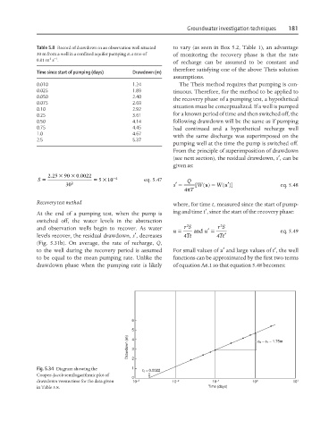
Fig. 5.34 Diagram showing the 2 1 t 0 = 0.0022 •
Cooper–Jacob semilogarithmic plot of
0
drawdown versus time for the data given 10 −3 10 −2 10 −1 10 0 10 1
in Table 5.8. Time (days)