Page 199 - Hydrogeology Principles and Practice

HYDC05 12/5/05 5:35 PM Page 182

182 Chapter Five

=
s′ . 23 Q log 10 t eq. 5.50
4π T t′
Hence, a plot of residual drawdown, s′, versus the
logarithm of t/t′ should provide a straight line. The
gradient of the line equals 2.3Q/4πT so that ∆s′,
the change in residual drawdown over one log cycle
of t/t′, enables a value of transmissivity to be found
from:

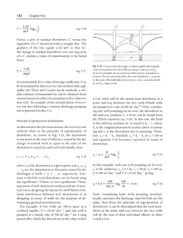
Fig. 5.35 Cross-section through a confined aquifer showing the
=
T . 23 Q eq. 5.51 cones of depression for two wells pumping at rates Q and Q .
2
1
4π∆ s′ From the principle of superposition of drawdown, at position A
between the two pumping wells, the total drawdown, s , is given
t
by the sum of the individual drawdowns s and s associated with
It is not possible for a value of storage coefficient, S, to 1 2
Q and Q , respectively.
2
1
be determined by this recovery test method although,
unlike the Theis and Cooper–Jacob methods, a reli-
able estimate of transmissivity can be obtained from
measurements in either the pumping well or observa- 0.5 m, what will be the steady-state drawdown at a
tion well. An example of the interpretation of recov- point mid-way between the two wells if both wells
3
−1
ery test data following a constant discharge pumping are pumped at a rate of 500 m day ? First, consider-
test is presented in Box 5.2. ing one well pumping on its own, the drawdown at
the mid-way position (r = 50 m) can be found from
1
the Thiem equation (eq. 5.28). In this case, the head
Principle of superposition of drawdown
at the mid-way position (h ) is equal to h − s where
1 o 1
As discussed in the previous section, the recovery test h is the original piezometric surface prior to pump-
o
method relies on the principle of superposition of ing and s is the drawdown due to pumping. There-
1
drawdown. As shown in Fig. 5.35, the drawdown fore, s = h − h . Similarly, s = h − h at r = 100 m
1 o 1 2 o 2 2
at any point in the area of influence caused by the dis- and equation 5.28 becomes, expressed in terms of
charge of several wells is equal to the sum of the drawdown:
drawdowns caused by each well individually, thus:
s − s = Q log r 2 eq. 5.53
s = s + s + s + ... + s eq. 5.52 1 2 2π T e r
t 1 2 3 n 1
where s is the drawdown at a given point and s , s , s In this example, with one well pumping on its own,
t 1 2 3
... s are the drawdowns at this point caused by the s is the unknown, s = 0.5 m, r = 50 m, r = 100 m,
1
1
2
2
n 3 −1 2 −1
discharges of wells 1, 2, 3... n, respectively. Solu- Q = 500 m day and T = 110 m day giving:
tions to find the total drawdown can be found using
the equilibrium (Thiem) or non-equilibrium (Theis) 500 100
05 +
.
s = . log e = 10 m eq. 5.54
π
1
equations of well drawdown analysis and are of prac- 2 110 50
tical use in designing the layout of a well-field to min-
imize interference between well drawdowns or in Now, considering both wells pumping simultan-
designing an array of wells for the purpose of de- eously, and since the discharge rates for both are the
watering a ground excavation site. same, then from the principle of superposition of
For example, if two wells are 100 m apart in a drawdown, it can be determined that the total draw-
2
−1
confined aquifer (T = 110 m day ) and one well is down at the point mid-way between the two wells
3
pumped at a steady rate of 500 m day −1 for a long will be the sum of their individual effects, in other
period after which the drawdown in the other well is words 2.0 m.