Page 194 - Hydrogeology Principles and Practice

HYDC05 12/5/05 5:35 PM Page 177

Groundwater investigation techniques 177

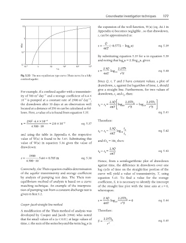
10 the expansion of the well function, W(u) (eq. A6.1 in
Appendix 6) becomes negligible , so that drawdown,
s, can be approximated as:
1
W(u) s Q (−0 .5772 log e u) eq. 5.39
=
−
4π T
10 −1
By substituting equation 5.35 for u in equation 5.39
and noting that log u = 2.3log u, gives:
e 10
10 −2
10 −1 1 10 10 2 10 3 10 4
s = log 10 eq. 5.40
1/u . 23 Q . 225 Tt
2
4π T rS
Fig. 5.33 The non-equilibrium type curve (Theis curve) for a fully
confined aquifer.
Since Q, r, T and S have constant values, a plot of
drawdown, s, against the logarithm of time, t, should
give a straight line. Furthermore, for two values of
For example, if a confined aquifer with a transmissiv-
ity of 500 m day and a storage coefficient of 6.4 × drawdown, s and s , then:
1
2
2
−1
3
−1
10 −4 is pumped at a constant rate of 2500 m day , 23 Q ⎡ 225 Tt 2 25 Tt ⎤
.
.
.
the drawdown after 10 days at an observation well s − s = ⎢ log 2 − log 1 ⎥
2 1 4π 10 2 10 2
located at a distance of 250 m can be calculated as fol- T ⎣ rS rS ⎦
lows. First, a value of u is found from equation 5.35: eq. 5.41
. 10
×
=
= 20
u 250 2 ⋅ 6 4 × −4 . 10 −3 eq. 5.37 Therefore:
⋅
. 4 500 10 23 Q t
.
s − s = log 2 eq. 5.42
2 1 4π 10
and using the table in Appendix 6, the respective T t 1
value of W(u) is found to be 5.64. Substituting this
and if t = 10t then:
value of W(u) in equation 5.36 gives the value of 2 1
drawdown: 23 Q
.
s − s = eq. 5.43
2
1
4π T
2500
=
=
4
6
0
s 5 . .705 m eq. 5.38
⋅
. 4 500 10 Hence, from a semilogarithmic plot of drawdown
against time, the difference in drawdown over one
Conversely, the Theis equation enables determination log cycle of time on the straight-line portion of the
of the aquifer transmissivity and storage coefficient curve will yield a value of transmissivity, T, using
by analysis of pumping test data. The Theis non- equation 5.43. To find a value for the storage
equilibrium method of analysis is based on a curve coefficient, S, it is necessary to identify the intercept
matching technique. An example of the interpreta- of the straight line plot with the time axis at s = 0,
tion of pumping test from a constant discharge test is whereupon:
given in Box 5.2.
=
=
s . 23 Q log 10 . 225 2 Tt 0 0 eq. 5.44
Cooper–Jacob straight-line method 4π T rS
A modification of the Theis method of analysis was Therefore:
developed by Cooper and Jacob (1946) who noted
that for small values of u (u < 0.01) at large values of S = . 225 Tt 0 eq. 5.45
time, t, the sum of the series beyond the term log u in r 2
e