Page 192 - Hydrogeology Principles and Practice

HYDC05 12/5/05 5:35 PM Page 175

Groundwater investigation techniques 175

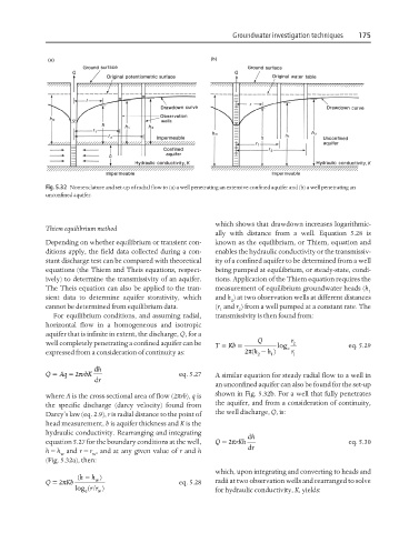
Fig. 5.32 Nomenclature and set-up of radial flow to (a) a well penetrating an extensive confined aquifer and (b) a well penetrating an
unconfined aquifer.

which shows that drawdown increases logarithmic-
Thiem equilibrium method
ally with distance from a well. Equation 5.28 is
Depending on whether equilibrium or transient con- known as the equilibrium, or Thiem, equation and
ditions apply, the field data collected during a con- enables the hydraulic conductivity or the transmissiv-
stant discharge test can be compared with theoretical ity of a confined aquifer to be determined from a well
equations (the Thiem and Theis equations, respect- being pumped at equilibrium, or steady-state, condi-
ively) to determine the transmissivity of an aquifer. tions. Application of the Thiem equation requires the
The Theis equation can also be applied to the tran- measurement of equilibrium groundwater heads (h
1
sient data to determine aquifer storativity, which and h ) at two observation wells at different distances
2
cannot be determined from equilibrium data. (r and r ) from a well pumped at a constant rate. The
1 2
For equilibrium conditions, and assuming radial, transmissivity is then found from:
horizontal flow in a homogeneous and isotropic
aquifer that is infinite in extent, the discharge, Q, for a
=
well completely penetrating a confined aquifer can be T Kb Q log e r 2 eq. 5.29
=
expressed from a consideration of continuity as: 2π h ( − h 1 ) r 1
2
=
=
Q Aq 2π r bK h d eq. 5.27 A similar equation for steady radial flow to a well in
r d
an unconfined aquifer can also be found for the set-up
where A is the cross-sectional area of flow (2πrb), q is shown in Fig. 5.32b. For a well that fully penetrates
the specific discharge (darcy velocity) found from the aquifer, and from a consideration of continuity,
Darcy’s law (eq. 2.9), r is radial distance to the point of the well discharge, Q, is:
head measurement, b is aquifer thickness and K is the
hydraulic conductivity. Rearranging and integrating h d
=
equation 5.27 for the boundary conditions at the well, Q 2π rKh eq. 5.30
h = h and r = r , and at any given value of r and h r d
w w
(Fig. 5.32a), then:
which, upon integrating and converting to heads and
−
=
w
Q 2π Kb h ( h ) eq. 5.28 radii at two observation wells and rearranged to solve
/
log ( rr )
e w for hydraulic conductivity, K, yields: