Page 53 - Hydrogeology Principles and Practice

HYDC02 12/5/05 5:38 PM Page 36

36 Chapter Two

BO X
Continued
2.3

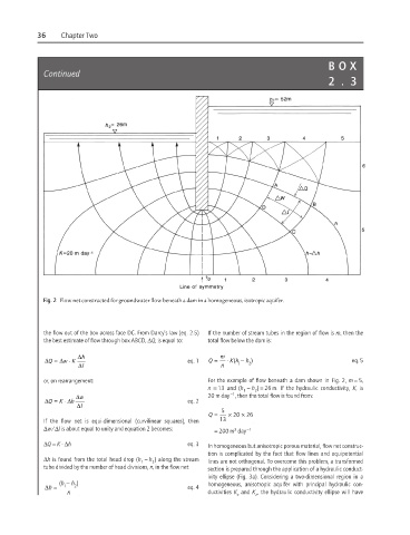
Fig. 2 Flow net constructed for groundwater flow beneath a dam in a homogeneous, isotropic aquifer.

the flow out of the box across face DC. From Darcy’s law (eq. 2.5) If the number of stream tubes in the region of flow is m, then the
the best estimate of flow through box ABCD, ∆Q, is equal to: total flow below the dam is:

⋅
=

(

∆Q ∆w K ∆h eq. 1 Q = m ⋅ Kh − h 2 ) eq. 5
1
∆l n
or, on rearrangement: For the example of flow beneath a dam shown in Fig. 2, m = 5,
n = 13 and (h − h ) = 26 m. If the hydraulic conductivity, K, is
1 2
−1
20 m day , then the total flow is found from:
=
∆Q K ⋅ ∆h ∆w eq. 2
∆l
×
=
×
Q 5 20 26
If the flow net is equi-dimensional (curvilinear squares), then 13
∆w/∆l is about equal to unity and equation 2 becomes:
3
= 200 m day −1
∆Q = K ⋅∆h eq. 3 In homogeneous but anisotropic porous material, flow net construc-
tion is complicated by the fact that flow lines and equipotential
∆h is found from the total head drop (h − h ) along the stream
1 2 lines are not orthogonal. To overcome this problem, a transformed
tube divided by the number of head divisions, n, in the flow net: section is prepared through the application of a hydraulic conduct-
ivity ellipse (Fig. 3a). Considering a two-dimensional region in a
h ( − h )
∆h = 1 2 eq. 4 homogeneous, anisotropic aquifer with principal hydraulic con-
n ductivities K and K , the hydraulic conductivity ellipse will have
x
z