Page 151 - Innovations in Intelligent Machines

142 A. Pongpunwattana and R. Rysdyk
4 4
step = 6 step = 20
3.5 time = 600 3.5 time = 2000
3 2.5 3
Latitude (deg) 1.5 2 1 1 Latitude (deg) 1.5 2 1 1
2.5

1 1
0.5 0.5
0 0
10 10.5 11 11.5 12 12.5 13 13.5 14 14.5 15 10 10.5 11 11.5 12 12.5 13 13.5 14 14.5 15
Longitude (deg) Longitude (deg)
(a) (b)
4 4
step = 27 step = 39
3.5 3.5
time = 2700 3 time = 3900
3
Latitude (deg) 2.5 2 1 1 Latitude (deg) 2.5 2 1 1

1.5
1 1.5 1
0.5 0.5
0 0
10 10.5 11 11.5 12 12.5 13 13.5 14 14.5 15 10 10.5 11 11.5 12 12.5 13 13.5 14 14.5 15
Longitude (deg) Longitude (deg)
(c) (d)
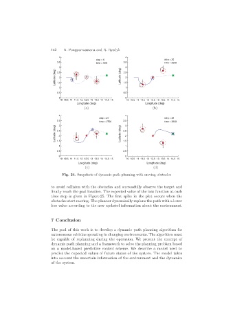
Fig. 24. Snapshots of dynamic path planning with moving obstacles

to avoid collision with the obstacles and successfully observe the target and
finally reach the goal location. The expected value of the loss function at each
time step is given in Figure 25. The first spike in the plot occurs when the
obstacles start moving. The planner dynamically replans the path with a lower
loss value according to the new updated information about the environment.

7 Conclusion

The goal of this work is to develop a dynamic path planning algorithm for
autonomous vehicles operating in changing environments. The algorithm must
be capable of replanning during the operation. We present the concept of
dynamic path planning and a framework to solve the planning problem based
on a model-based predictive control scheme. We describe a model used to
predict the expected values of future states of the system. The model takes
into account the uncertain information of the environment and the dynamics
of the system.