Page 148 - Innovations in Intelligent Machines

Evolution-based Dynamic Path Planning for Autonomous Vehicles 139
4 4
step = 5 step = 14
3.5 time = 500 3.5 time = 1400
3 3
Latitude (deg) 2.5 2 1 1 2 Latitude (deg) 2.5 2 1 1 2

1.5
1.5
1 2 1 2
0.5 0.5
0 0
10 10.5 11 11.5 12 12.5 13 13.5 14 14.5 15 10 10.5 11 11.5 12 12.5 13 13.5 14 14.5 15
Longitude (deg) Longitude (deg)
(a) (b)

4 4
step = 22 step = 34
3.5 time = 2200 3.5 time = 3400
3 2.5 3
Latitude (deg) 1.5 2 1 1 2 2 Latitude (deg) 1.5 2 1 1 2 2
2.5

1 1
0.5 0.5
0 0
10 10.5 11 11.5 12 12.5 13 13.5 14 14.5 15 10 10.5 11 11.5 12 12.5 13 13.5 14 14.5 15
Longitude (deg) Longitude (deg)
(c) (d)

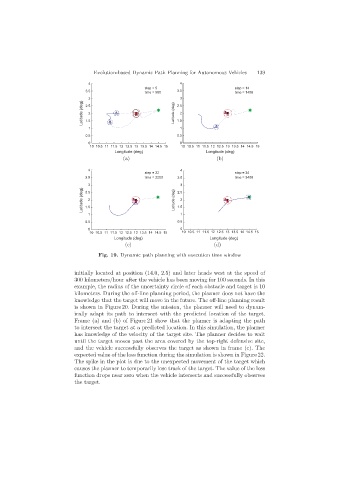
Fig. 19. Dynamic path planning with execution time window

initially located at position (14.0, 2.5) and later heads west at the speed of
300 kilometers/hour after the vehicle has been moving for 100 seconds. In this
example, the radius of the uncertainty circle of each obstacle and target is 10
kilometers. During the off-line planning period, the planner does not have the
knowledge that the target will move in the future. The off-line planning result
is shown in Figure 20. During the mission, the planner will need to dynam-
ically adapt its path to intersect with the predicted location of the target.
Frame (a) and (b) of Figure 21 show that the planner is adapting the path
to intersect the target at a predicted location. In this simulation, the planner
has knowledge of the velocity of the target site. The planner decides to wait
until the target moves past the area covered by the top-right defensive site,
and the vehicle successfully observes the target as shown in frame (c). The
expected value of the loss function during the simulation is shown in Figure 22.
The spike in the plot is due to the unexpected movement of the target which
causes the planner to temporarily lose track of the target. The value of the loss
function drops near zero when the vehicle intersects and successfully observes
the target.