Page 145 - Innovations in Intelligent Machines

136 A. Pongpunwattana and R. Rysdyk
4 step = 9 4 step = 22
time = 900 time = 2200
3.5 3 3.5 3
Latitude (deg) 2.5 2 1 1 1 Latitude (deg) 2.5 2 1 1

1.5
1 1 1.5 1 1 1
0.5 0.5
0 0
10 10.5 11 11.5 12 12.5 13 13.5 14 14.5 15 10 10.5 11 11.5 12 12.5 13 13.5 14 14.5 15
Longitude (deg) Longitude (deg)
(a) (b)

4 4
step = 46 step = 56
3.5 time = 4600 3.5 time = 5600
3 3
Latitude (deg) 2.5 2 1 1 1 Latitude (deg) 2.5 2 1 1 1

1.5
1 1 1.5 1 1
0.5 0.5
0 0
10 10.5 11 11.5 12 12.5 13 13.5 14 14.5 15 10 10.5 11 11.5 12 12.5 13 13.5 14 14.5 15
Longitude (deg) Longitude (deg)
(c) (d)
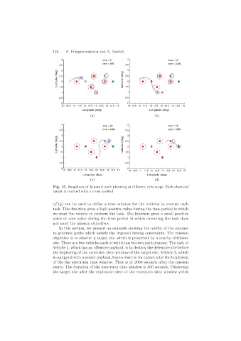
Fig. 15. Snapshots of dynamic path planning at different time steps. Each observed
target is marked with a cross symbol

F
α (q) can be used to define a time window for the vehicles to execute each
i
task. This function gives a high positive value during the time period in which
we want the vehicle to perform the task. The function gives a small positive
value or zero value during the time period in which executing the task does
not meet the mission objectives.
In this section, we present an example showing the ability of the planner
to generate paths which satisfy the imposed timing constraints. The mission
objective is to observe a target site which is protected by a nearby defensive
site. There are two vehicles each of which has its own path planner. The task of
Vehicle 1, which has an offensive payload, is to destroy the defensive site before
the beginning of the execution time window of the target site. Vehicle 2, which
is equipped with a sensor payload, has to observe the target after the beginning
of the the execution time window. That is at 2000 seconds after the mission
starts. The duration of the execution time window is 500 seconds. Observing
the target site after the expiration time of the execution time window yields