Page 144 - Innovations in Intelligent Machines

Evolution-based Dynamic Path Planning for Autonomous Vehicles 135
uses it as the basis to compute new solutions even though the new problem
is slightly different from the previous problem. This takes an advantage of
evolutionary algorithms that several candidate solutions are available at any
time during the optimization process.
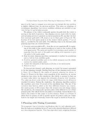
The planner of the vehicle continually updates its path while the vehicle is
moving in the field of operation. The planning process starts with the static
path planning process to generate an initial population P 0 and find the first
best candidate path Q(0) ∈ P 0 depicted as the black path in Figure 14. The
V
z
location of the first spawn point is at the desired vehicle position ¯ (s 1 )at
specified by the path Q(0). The following steps in the dynamic path
time t s 1
planning algorithm are described below
1. Generate a new population P i+1 from the current population P i by updat-
ing all the paths in the current population to begin at the location of the
next spawn point. The paths are modified by removing a small number of
segments from the start of the paths and adding other segments to join
the paths to the spawn point.
2. Run the static planning algorithm continuously to update the population
and to find the best candidate path.
3. Send the updated candidate path to the vehicle navigator once the vehicle
reaches the current spawn point.
4. Update the estimates of the locations of sites in the environment.
5. Return to step 1
To demonstrate dynamic path planning, we revisit the scenario presented
in the last planning example. Starting from the off-line planning result shown
in frame (d) of Figure 12, the results of dynamic planning are shown in
Figure 15. Frames in the figure show snapshots of the simulation at various
simulation time steps. In this simulation, the vehicle is assumed to have an
on-board radar which can improve the estimates of nearby sites’ locations.
The radar can detect a site within the range of 60 kilometers with 40 meters
standard deviation. During the simulation, the planning algorithm updates
the candidate path every 10 seconds of the simulation time. The size of the
execution time horizon, which is the time difference between two consecu-
tive spawn points, is 100 seconds. Since the scenario does not change during
the simulation, the dynamically updated path is little different to the off-line
planned path. The vehicle follows the path to successfully observe the first two
targets, but misses the last target in its first attempt. Frame (c) of Figure 15
shows that the planner is able to quickly update the path to guide the vehicle
back to the target and eventually observe the target as shown in Frame (d).

5 Planning with Timing Constraints

To incorporate time-of-execution specifications into the path planning prob-
F
lem, the task score weighting factor α used in the objective function is defined
i
as a time-dependent function. This time-dependent score weighting function