Page 147 - Innovations in Intelligent Machines

138 A. Pongpunwattana and R. Rysdyk
150 vehicle1
Expected value of loss function 120
140
vehicle2
130

110
100
90

80
70
0 50 100 150
Generation
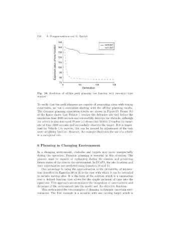
Fig. 18. Evolution of off-line path planning loss function with execution time
window

To verify that the path planners are capable of generating plans with timing
constraints, we ran a simulation starting with the off-line planning results.
The dynamic planning simulation results are shown in Figure 19. Frame (b)
of the figure shows that Vehicle 1 reaches the defensive site well before the
simulation time 2000 seconds and successfully destroys the obstacle, although
the vehicle is also destroyed. Frame (c) shows that Vehicle 2 reaches the target
site at time 2200 seconds and successfully observes the target. If it is impor-
tant for Vehicle 1 to survive, this can be insured by adjustment of the task
score weighting function. However, the example illustrates the use of a vehicle
in a sacrificial role.

6 Planning in Changing Environment

In a changing environment, obstacles and targets may move unexpectedly
during the operation. Dynamic planning is essential in this situation. The
planner must be capable of replanning during the mission and predicting
future states of the sites in the environment. In ECoPS, the site locations and
their uncertainties are predicted using Equation 10 and 11.
One advantage in using the approximation to the probability of intersec-
tion described in Equation 30 or 31 is the ease with which it can be extended
to include moving sites. It is the form of the solution which is a summation
over a defined function that allows for the simple inclusion of time into the
equations. This approach accommodates the integration of uncertainties and
dynamics of the environment into the model and the objective function.
This section provides two examples of planning in dynamic uncertain envi-
ronments. The first example is a scenario with one moving target which is