Page 40 - Innovations in Intelligent Machines

28 M.L. Cummings et al.
1 event # of UAVs events
Arrival rate = λ =# of UAVs ∗ = (6)
(NT + IT) NT + IT time
In terms of the service rate, by definition, the operator takes, on average, an
IT length of time to process each event. Therefore assuming that the operator
can constantly service events (i.e., does not take a break while events are in
the queue):
1 events
Service rate = µ = (7)
IT time
By using Little’s theorem, we can show that the mean time an event spends
in the queue is:
λ/µ
W q = (8)
µ − λ
For the purposes of our predictive model, we will assume that this wait
time in the queue (Wq, eqn. 8) includes both situation awareness wait times
(WTSA) as well as wait times due to operator engagement in another task
(referred to as WTQ in the previous section).
Now that we have established our operator model based on queuing theory,
we will now show how this human model can be used to determine operator
capacity predictions through simulated annealing optimization.

3.6 Optimization through Simulated Annealing

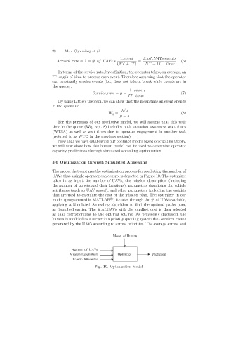
The model that captures the optimization process for predicting the number of
UAVs that a single operator can control is depicted in Figure 10. The optimizer
takes in as input the number of UAVs, the mission description (including
the number of targets and their locations), parameters describing the vehicle
attributes (such as UAV speed), and other parameters including the weights
that are used to calculate the cost of the mission plan. The optimizer in our
R
model (programmed in MATLAB ) iterates through the # of UAVs variable,
applying a Simulated Annealing algorithm to find the optimal paths plan,
as described earlier. The # of UAVs with the smallest cost is then selected
as that corresponding to the optimal setting. As previously discussed, the
human is modeled as a server in a priority queuing system that services events
generated by the UAVs according to arrival priorities. The average arrival and

Model of Human

Number_of_UAVs
Mission Description Optimizer Prediction
Vehicle Attributes
Fig. 10. Optimization Model