Page 42 - Innovations in Intelligent Machines

30 M.L. Cummings et al.
Table 3. Constraints for Simulated Annealing
Constraints
• A UAV cannot visit targets for which it cannot
meet the times on target
• Each UAV must visit at least one target
• UAV routes must start and end at launch
locations.

14000

12000

10000
Mission cost 8000

6000

4000

2000
1 2 3 4 5 6 7 8 9 10
#UAVs used
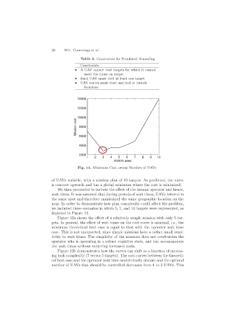
Fig. 11. Minimum Cost versus Number of UAVs

of UAVs variable, with a mission plan of 10 targets. As predicted, the curve
is concave upwards and has a global minimum where the cost is minimized.
We then proceeded to include the effect of the human operator and hence,
wait times. It was assumed that during periods of wait times, UAVs loitered in
the same spot and therefore maintained the same geographic location on the
map. In order to demonstrate how plan complexity could affect the problem,
we included three scenarios in which 5, 7, and 10 targets were represented, as
depicted in Figure 12.
Figure 12a shows the effect of a relatively simple mission with only 5 tar-
gets. In general, the effect of wait times on the cost curve is minimal, i.e., the
minimum theoretical best case is equal to that with the operator wait time
case. This is not unexpected, since simple missions have a rather small sensi-
tivity to wait times. The simplicity of the missions does not overburden the
operator who is operating in a robust cognitive state, and can accommodate
the wait times without incurring increased costs.
Figure 12b demonstrates how the curves can shift as a function of increas-
ing task complexity (7 versus 5 targets). The cost curves between the theoreti-
cal best case and the operator wait time model clearly deviate and the optimal
number of UAVs that should be controlled decreases from 4 to 3 UAVs. This