Page 41 - Innovations in Intelligent Machines

Predicting Operator Capacity for Supervisory Control of Multiple UAVs 29
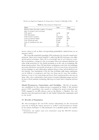
Table 2. Optimization Parameters
Name Unit Value
Mission Data (includes number of targets, - 5–10 targets
time on targets, and locations)
UAV speed mi/hr 100
UAV Endurance hr 5
UAVs launch location Cartesian 0,0
Cost per missed target $/target 1500
Cost of fuel per min $/min 10
Cost of operations per min $/min 1
NT min 3 2
IT min 0.3 1

service rates as well as their corresponding probabilistic distributions are as
assumed earlier.
We chose the simulated annealing (SA) technique for heuristic-based opti-
mization. There were several benefits to selecting the SA technique over other
optimization techniques. First, SA is a technique that is well suited to avoid-
ing local minima, a property that is necessary when sub-optimal solutions can
exist while searching for the global optimum as is the case in evaluating dif-
ferent mission plans. Also, SA introduces randomness such that the technique
generates alternative acceptable solutions on different runs, hence allowing the
system designer to seek alternative optimal designs when initial solutions are
not feasible. Two limitations of SA are that problems with many constraints
can be difficult to implement and that run times can be long. Our problem,
however, is one of few constraints and hence their implementation was not an
issue. Also, since optimization takes place in mission planning stages and not
in time-critical mission replanning, the long run times have a minimal adverse
effect.

Model Parameters, Constraints, and Variables. The list of parame-
ters established for the design process is presented in Table 2. We selected
generic UAV capabilities that would be exhibited by small-to-medium size
UAVs engaged in an ISR mission such as the Hunter or Shadow. Our cost
function was discussed previously (5) and Table 3 details the constraints used
in our model.

3.7 Results of Simulation
We first investigated the cost-UAV number relationship for the theoretical
best case in which the human operator is “perfect” and introduces no delays
in the system. In Figure 11, the optimized cost is plotted against the number

2
Interaction and neglect times were determined using the MAUVE interface
described previously.