Page 231 - Materials Chemistry, Second Edition

L1644_C05.fm Page 204 Monday, October 20, 2003 12:02 PM

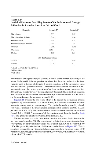
TABLE 5.14
Statistical Parameter Describing Results of the Environmental Damage
Estimation in Scenarios 1 and 2 as External Costs a

Parameter Scenario 1 b Scenario 2 c
Normal mean 3.73 0.87
Normal standard deviation 5.16 1.08
Geometric mean 2.19 0.55
Geometric standard deviation 2.81 2.62
Minimum 0.087 0.029
Maximum 221.7 74.4
Median 2.09 0.53

68% Confidence interval
Superior 6.15 1.44
Inferior 0.78 0.21
a mU.S.$ per kWh (1E-3 U.S.$/kWh).
b Without filters.
c With filters.

been made in one separate run per scenario. Because of the inherent variability of the
Monte Carlo model, it is not possible to affirm that the set of values for the input
variables used in the run of Scenario 2 (current situation) will be the same as those
used in Scenario 1 (former situation). The same was done with the calculation of LCI
uncertainties and, due to the generation of random numbers, every run occurs in a
different way. In order to verify the importance of this variability on the final outcome,
both simulations have also been made in one run; it could be checked that the results
are the same because the variations are negligible.
Figure 5.16 presents the first result, which is the case of the incineration process
supported by the advanced AGTS. In the x-axis, it is possible to observe the envi-
ronmental damage cost per energy output. The y-axis shows the probability of each
cost value. The mean of the environmental damage cost in Scenario 2 is 0.87 mU.S.$
per kWh (with m = 10 ). The total number of iterations carried out with the software
–3
Crystal Ball is 10,000. A summary of all the results generated can be found in Table
5.14. The geometric standard deviation from them is 2.62.
The second case occurs in time before the first one, when the incinerator did
not have an advanced AGTS. The emissions of pollutants were more important and
consequently the environmental damage cost is much higher, with 3.73 mU.S.$ per
kWh. The probability distribution of this result can be found in Figure 5.17. This is
explained because the only important change corresponds to the mean values of 10
parameters, including pollutants and electricity production, which are lower with an
advanced AGTS installed.

© 2004 CRC Press LLC