Page 232 - Materials Chemistry, Second Edition

L1644_C05.fm Page 205 Monday, October 20, 2003 12:02 PM

Prevision: External Environmental Costs
for Scenario 2 "With Filters"
.080 800
Probability .060 600 Frequency

.040
400
.020

.000 200
0
0.0000 1.5000 3.0000 4.5000 6.0000
mU.S.$/kWh
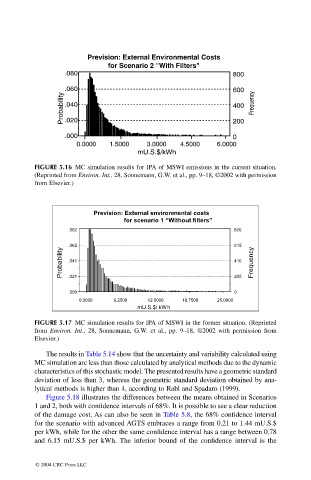
FIGURE 5.16 MC simulation results for IPA of MSWI emissions in the current situation.
(Reprinted from Environ. Int., 28, Sonnemann, G.W. et al., pp. 9–18, ©2002 with permission
from Elsevier.)

Prevision: External environmental costs
for scenario 1 “Without filters”
.082 820
.062 615
Probability .041 410 Frequency

205
.021
.000 0
0.0000 6.2500 12.5000 18.7500 25.0000
mU.S.$/ kWh

FIGURE 5.17 MC simulation results for IPA of MSWI in the former situation. (Reprinted
from Environ. Int., 28, Sonnemann, G.W. et al., pp. 9–18, ©2002 with permission from
Elsevier.)
The results in Table 5.14 show that the uncertainty and variability calculated using
MC simulation are less than those calculated by analytical methods due to the dynamic
characteristics of this stochastic model. The presented results have a geometric standard
deviation of less than 3, whereas the geometric standard deviation obtained by ana-
lytical methods is higher than 4, according to Rabl and Spadaro (1999).
Figure 5.18 illustrates the differences between the means obtained in Scenarios
1 and 2, both with confidence intervals of 68%. It is possible to see a clear reduction
of the damage cost. As can also be seen in Table 5.8, the 68% confidence interval
for the scenario with advanced AGTS embraces a range from 0.21 to 1.44 mU.S.$
per kWh, while for the other the same confidence interval has a range between 0.78
and 6.15 mU.S.$ per kWh. The inferior bound of the confidence interval is the

© 2004 CRC Press LLC