Page 131 - Integrated Wireless Propagation Models

I
M a c r o c e I P r e d i c t i o n M o d e I s - P a r t 2 : P o i n t - t o - P o i n t M o d e I s 109
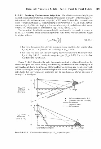
3.1.2.3.2 Calculating Effective Antenna Height Gain The effective antenna height gain
calculation considers the terrain contour and the relation of effective antenna height (he)
to the standard condition antenna height (h1) of 100 feet (-30.5 m). The Lee model con­
siders four different cases: (1) terrain sloping is upward when he > hl' (2) over a flat ter­
rain when he > hl' (3) terrain sloping is downward when he < hl' and ( 4) over a flat terrain
when he < h1• These cases are illustrated in Figs. 3.1.2.3.1 and 3.1.2.3.2.
The formula of the effective antenna height gain from the Lee model is shown in
Eq. (3.1.2.3) when the actual antenna height is the same as the standard antenna height
(h; = h1) as follows:

(3 1 . 2.3.1)
.

1 . For these two cases (for a terrain sloping upward and for a flat terrain when
he > h1), Eq. (3.1.2.3.1) results in a positive gain (G effi' > 0 dB).
2. For these two cases (for a terrain sloping downward and for a flat terrain when
he < h1), Eq. (3.1.2.3.1) results in a negative gain (Ge ' < 0 dB). If he < hJ10, then
f fi
/
he is forced to cap at h 1 0.
Figure 3.1.2.3.3 illustrates the path loss prediction that is obtained based on the
area-to-area path loss curve, adding or subtracting the effective antenna height gain at
each local point due to the influence of the local terrain contour; as a result, the overall
point-to-point signal strength prediction is plotted for each local point along the mobile
path. Note that the variation in prediction can be significant, as shown at points D
through G in the figure.

Geffh > 0 i
h

for terrain h e
sloping up

.,.,... Diffuse reflection point (R 1 )
..,..... •
.,.,... • Specular reflection point (R2)
v --- Direct wave
- - - Specular wave
-·· ···· ····· Diffuse wave
h ,
l
Ge ffh > 0 for h e
flat terrain
when h e > h 1

FIGURE 3.1.2.3.1 Effective a n tenna height gain (Getth)-positive gai n .