Page 135 - Integrated Wireless Propagation Models

M a c r o c e l l P r e d i c t i o n M o d e l s - P a r t 2 : P o i n t - t o - P o i n t M o d e l s 113

3 . 1 . 2.4.3 Multiple-Knife-Edge Case with Single-Knife-Edge Check When a signal path
is blocked by multiple knife edges, the Lee model compares diffraction losses
calculated by adding all knife edges together and from each one separately. The great­
est loss value is then used for the diffraction loss component of the signal strength
prediction.
The multiple-knife-edge evaluation involves these steps:

1. For each knife edge, the Lee model calculates the obstruction height (h ) using
P
the Epstein-Petersen method (see Sec. . 9.2.2.2). The Lee models consider two
1
different scenarios-when there are two knife edges and when there are three
or more knife edges.
2. The parameter v is evaluated for each single knife edge, assuming no other
knife edge, and the individual single-knife-edge diffraction loss is computed
from the appropriate formula in Table 3.1.2.4.1.
3. The individual values L; of two or three knife edges are calculated as shown in
Fig. . 9.2.2.2.2, and the individual values are summed for all knife edges as a
1
1
total diffraction loss (q using the formulas in Table 3.1.2.4. .
4. The "single-knife-edge check" s then used o compare the greatest diffraction
i
t
loss caused by any individual knife edge with the total diffraction loss. The
Lee model uses the greatest of these values for the diffraction loss component
of the signal strength prediction. This ensures that the total loss caused by the
multiple-knife-edge calculation is at least as great as the loss caused by any one
knife edge considered individually.

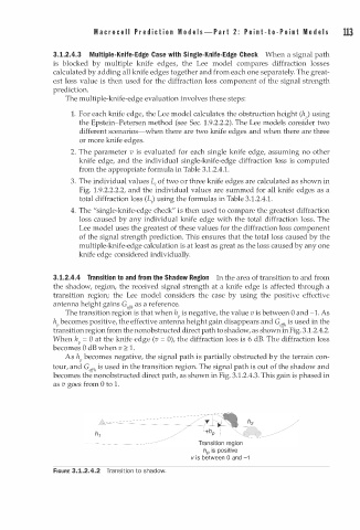
3.1.2.4.4 Transition to and from the Shadow Region In the area of transition to and from
the shadow, region, the received signal strength at a knife edge is affected through a
transition region; the Lee model considers the case by using the positive effective
antenna height gains G as a reference.
,ft7
v
The transition region is that when h is negative, the value i s between 0 and -1. As
P
h becomes positive, the effective antenna height gain disappears and G is used in the
,ff"
P
transition region from the nonobstructed direct path to shadow, as shown in Fig. 3.1.2.4.2.
When h P = 0 at the knife edge (v = 0), the diffraction loss is 6 dB. The diffraction loss
becomes 0 dB when v :2: 1 .
b
A s h becomes negative, the signal path s partially obstructed y the terrain con­
i
P
tour, and G is used in the transition region. The signal path is out of the shadow and
,11,,
becomes the nonobstructed direct path, as shown in Fig. 3.1.2.4.3. This gain is phased in
as v goes from 0 to .
1
� �
� /
,f�=========: ;q �li ::i-: : 1 f �� n ,'"::c
ra io � //
hP is positive
v is between 0 and -1
FIGURE 3.1.2.4.2 Transition to shadow.