Page 138 - Integrated Wireless Propagation Models

116 C h a p t e r T h r e e

Base
Station -67.0 dBm -68.0 dBm -69.5 dBm Raw prediction
()------���------���------�@)-------�
Radial d;
Radial* (km)

A, = A B, = (A, + 8)/2 = C, = (B, + C)/2 = Smoothing
[-67.0 + (-68.0)]/2 [-67.5 + (-69.5)] /2 algorithm

Base
Station -67.0 dBm -67.5 dBm -68.5 dBm Final prediction
()�----�Qg-----�@9-----���--------J�
Radial d; Radial* (km)

*Note: radial dx and radial length are user inputs.
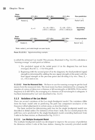
FIGURE 3.1.2.5.1 Signal-smoothn g example.
i

is called the enhanced Lee model. This process, illustrated in Fig. 3.1.2.5.1, calculates a
"running average" at each point as follows:
1. The predicted signal at the initial point (A in the diagram) has not been
averaged, thus let A , = A for this point.
2. Beginning with the second point (B in the diagram), the final predicted signal
strength is determined by adding the raw signal strength at this point with the
final signal strength at the previous point and dividing it by two. Thus, B, =
(A, + B)/2 and so on.

3.1.2.6.2 From the Measured Data We have to use the running average to get the local
means from the measured data. The local mean has been determined by averaging 50
samples of a piece of data over a distance of 40 wavelengths at 800 MHz. If the carrier
frequency is at 400 MHz, the averaging of a distance of 20 wavelengths is adequate. It
1
1
has been determined by Lee9 and described in Sec. . 6.3. .
o
3 . 1 . 3 Variations f the Lee Model
There are several variations of the Lee single breakpoint model. The variations differ
from the basic model only in predicting the path loss component (exclusive of the
frequency-offset adjustment) in certain areas, as described below.
The basic method for determining path loss for the single breakpoint model was
described in detail earlier. For distances of less than 1 mile, the Lee model projects the
path loss curve predicted by the single breakpoint model extending backward from
.
1 mile to the base station, as illustrated in Fig. 3.1.3 1 . 1 .
3 . 1 . 3 . 1 Lee Multiple Breakpoint Model
The multiple breakpoint model was developed to improve the accuracy of prediction
for distances within 1 mile of the base station. Among the currently provided model