Page 194 - Integrated Wireless Propagation Models

172 C h a p t e r T h r e e

� (\ - 1\

�
'\'-; / ,\) "';� \: 9
Possible knives: A, B, C, D, and E

Possible knives: B, C, and E

,------------< Calculate gain )----------,
and loss

B
--------------
i
__ .., _ _ _ _ __ _ _ _ _ _ _ _ _ __ _ _ _ _ _ _ _
h pB
Calculate diff loss due to h s• h c• h pE
p
p
Effh8 = 201og (�: )
� = 201og(:rc ) Total loss =
h ppc ppc Total gain = 0 loss8 + 0 lossc + 0 loss E
� = 201og(�) Effh +� +�
h ppE h ppE B h E h pp E
pp

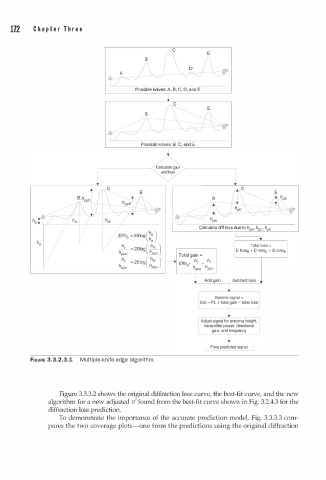
FIGURE 3.3.2.3.1 M u l tiple-knife-edge algorith .
m

Figure 3.3.3.2 shows the original diffraction loss curve, the best-fit curve, and the new
algorithm for a new adjusted v' found from the best-fit curve shown in Fig. 3.2.4.3 for the
diffraction loss prediction.
To demonstrate the importance of the accurate prediction model, Fig. 3.3.3.3 com­
pares the two coverage plots-one from the predictions using the original diffraction