Page 214 - Integrated Wireless Propagation Models

192 C h a p t e r F o u r

Therefore, we will use an empirical curve P0, which can be found by taking Pws from
curve (a) and adding the block loss Lb in curve (b) shown in Fig. 4.2.1.2.2 as our pre­
dicted curve to compare with the measured data. Again G A will be considered when
'
'
d > 200 . When d :;:; 200 , G A = 0.
1
1
The blockage length B shown in Fig. 4.2.1.2.3 is the sum of the widths of all build­
ings, which are located in line with the transmitted signal. The curve (b) in Fig. 4.2.1.2.2
shows that rapid attenuation occurred while B is less 500 ft. When B is greater 1000 ft,
a nearly constant value of 18 dB is observed. The corner turning effects were found
during the test. When the mobile turned from one street to another street, the signal
strength changed noticeably. Because the blockage length of the buildings varies quite
differently during the turning of the mobile from one street to another street, this sce­
1
nario can be taken care of in the model. The curve b is used for obtaining L8 in Eq. ( 4.2. . 2.1)
in the microcell prediction model.
In the microcell environment, the antenna height ha at the base station and antenna
.
gain Ga relationship follows a 9-dB I oct rule was observedY Therefore, G)n Eq. ( 4.2 1 . 2.1)
is shown as follows:
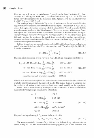
(4.2.1.2.4)

The numerical expression of two curves in Fig. 4.2.1.2.3 can be depicted as follows:
d � ' '
Pw - s - � - 7 7 dBm- 21.5log , + 30log , 100 :;:; d < 200
100 20
= P - 8 3.5 dBm- 1 4 l og g , +30log ;0, 200 :;:; d < 1000 ' (4.2.1.2.5)
'
1 0
= P - 9 3.3 dBm- 36.5log g , + 30log ;0, 1000 :;:; d < 5000 '
'
1 0
'
= use the macrocell prediction model for 5000 :;:; d
Readers may notice that the symbol i s for the distance in the microcell model and that the
d
symbol r is for the distance in the macrocell model. This makes it easier to recognize that
the prediction calculation is for the microcell or the macrocell model from the equations.
We set the maximum building blockage loss to 20 dB instead of 18 dB in the follow­
ing expression for giving a conservative estimation:
L = 0
B
= 1 +0.5 log B ,
10
B ' '
B
1
= . 2 + 12.5 log , 25 :;:; < 600 (4.2.1.2.6)
25
B ' '
= 7 .95+3 log , 600 :;:; B < 3000
1
600
= 2 0 dB 3000 :;:; B
The predicted signal strength P os shown in Eq. 4.2.1.2.1 is
1
p OS = P LOS + L + GA = P LOS + LA ( 4.2. . 2. 7)
B
'
The measurements for the case of d :;:; 200 were carried out along various routes, as
1
shown in Fig. 4.2.1.2.4. The measurement on the zigzag route (R2) in San Francisco was