Page 256 - Integrated Wireless Propagation Models

234 C h a p t e r F o u r

and

( 4.4.2.1.2)

Let's denote R"' as the measured result from the mobile for each local point and s as
the difference between our predicted result and the measured result at each local point.
Then we have

( 4.4.2.1.1)

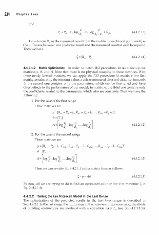
4.4.2.1.2 Matrix Optimization In order to match JLO procedure, let us make up our
matrices y, '0, and A. Note that there is no physical meaning to these matrices. With
these newly formed matrices, we can apply the JLO procedure. In matrix y, the first
matrix contains only the constant values, such as measured data and distance; in matrix
'0, the second one contains only the parameters, which can be fine-tuned and have
direct effects to the performance of our model; in matrix A, the third one contains only
the coefficients related to the parameters, which also are constants. Then we have the
following:
1. For the case of the first range
Three matrixes are

.
( 4.4.2 1 . 2)

2. For the case of the second range
Three matrixes are

( 4.4.2.1.3)

Then we can rewrite Eq. 4.4.2.1.1 into a matrix form as follows:

s = y - A-o ( 4.4.2.1.4)

By now, all we are trying to do is find an optimized solution for '0 to minimize s in
Eq. (4.4.2.1.4).

4.4.2.2 Tuning the Lee M i crocell Model in the Last Range
The optimization of the predicted results in the first two ranges is described in
Sec. 4.4.2.1. In the last range, the third range in the non-near-in zone scenario, the effects
of building obstructions are modeled with a correction term L8 (see Eq. (4.2.1.2.3)).