Page 261 - Integrated Wireless Propagation Models

M i c r o c e l l P r e d i c t i o n M o d e l s 239

4.5.2. 1 Dual-Slope Model
In a dual-slope model, two separate path loss exponents are used to characterize the prop­
agation, together with a breakpoint distance of a few hundred meters, at which propaga­
tion changes from one regime to the other. In this case, the path loss is modeled as

k
r ill for r :::; rb
1 k (4.5.2.1.1)
r for r > rb
r "
- r, b I
( r b r
or the path loss L in decibels

10n 1 log(f} L for r :::; rb
=l Y for r > rb
L Y (4.5.2.1.2)
10n2 log(f} L

where L is the reference path loss at r = rb' rb is the breakpoint distance between 100 and
Y 1
500 m, n is the path loss exponent for r :::; rb, and n is the path loss exponent for r > rb.
2
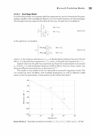
Typical values for the path loss exponents are found by measurement to be around
n = 2 and n = 4, with breakpoint distances of 200 to 500 m. However, these values vary
1
2
between different measurements, as discussed in. 20-22
This model is very similar to the Lee microcell-to-macrocell integration model. The
Lee model has more flexibility with multiple breakpoints as well as different radial
zones so that the granularity of data points can be further fine-tuned.
-20

-40

L -60
co
""0
._!...
(/) -80
(/)
.2
.s::.
(ti -1 00
[l_
-1 20

-1 40 2
1 0 0 1 0 1 1 0 1 0 3 1 0 4
Distance (m)
m
FIGURE 4.5.2.1.1 Dual-slope empirical loss models. n1 = 2 , n = 4, r" = 100 , and L, = 20 dB.
2