Page 350 - Integrated Wireless Propagation Models

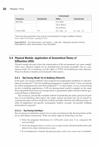
328 C h a p t e r F i v e

Environment
Frequency Residential Office Commercial
M
900 H z 9 (1 floor)
19 (2 floors)
24 (3 floors)
1.8-2.0 GHz 4n 15 + 4(n 1 ) 6 + 3(n 1 )
-
-
.
*Note that the penetration loss may be overestimated for large numbers of floors.
Source: T a ble 5.5.2.2 from,47 courtesy of ITU.
TABLE 5.5.2.2 Floor Penetration Loss Factors, L, (dB) with n Being the Number of Floors
I
Penetrated for n door Transmission Loss Calculation

5.6 Physical Models-Application of Geometrical Theory of
Diffraction { GTD)
Physical models are used when the characteristics of the environment vary more compli­
cated ways. Physical models can be classified into two kinds of models. One is a ray­
tracing model for in-building, and the other is FDTD (finite-difference time domain).
These two kinds of models are introduced in this section.

5.6.1 Ray-Tracing Model for In-Buil i n g P icocell)
d
(
In the past, ray-tracing methods were proposed for propagation prediction in microcel­
2
lular environments4S-5 and for modeling propagation in rough terrain. 3 Later, ray tracing
5
for indoor propagation has also been proposed.6.54-59 In this section, we are concentrating
for the in-building applications. A 3D ray-tracing-based model is applied on the same
floor using both brute force ray tracing based on geometrical optics and the uniform geo­
metrical theory of diffraction. 6 0
Ray tracing is a physically tractable method of predicting the delay spread and path
loss of an in-building radio signal. The delay spread and path loss can be found by
counting the time and loss of arrival of all the possible reflected and diffracted rays. In
order to implement site-specific propagation models, accurate site-specific building
information is required.

5.6. 1 . 1 Ray-Tracing Technique
Ray tracing is an exhaustive search of a ray tree accounting for the decomposition of the
ray at each planar intersection. There are many steps for searching a ray tree:

1. First, the program determines if a LOS path exists and, if so, computes the
received field.
2. Next, the program traces a source ray in a previously determined direction and
detects if an object intersection occurs.
3. If no intersection is found, the process stops, and a new source ray is initiated.