Page 182 - Intro to Tensor Calculus

177

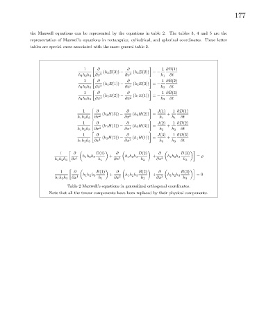
the Maxwell equations can be represented by the equations in table 2. The tables 3, 4 and 5 are the
representation of Maxwell’s equations in rectangular, cylindrical, and spherical coordinates. These latter
tables are special cases associated with the more general table 2.

1 ∂ ∂ 1 ∂B(1)
(h 3 E(3)) − (h 2 E(2)) = −
h 1 h 2 h 3 ∂x 2 ∂x 3 h 1 ∂t

1 ∂ ∂ 1 ∂B(2)
(h 1 E(1)) − (h 3 E(3)) = −
h 1 h 2 h 3 ∂x 3 ∂x 1 h 2 ∂t

1 ∂ ∂ 1 ∂B(3)
(h 2 E(2)) − (h 1 E(1)) = −
h 1 h 2 h 3 ∂x 1 ∂x 2 h 3 ∂t

1 ∂ ∂ J(1) 1 ∂D(1)
(h 3 H(3)) − (h 2 H(2)) = +
h 1 h 2 h 3 ∂x 2 ∂x 3 h 1 h 1 ∂t
1 ∂ ∂ J(2) 1 ∂D(2)
(h 1 H(1)) − (h 3 H(3)) = +
h 1 h 2 h 3 ∂x 3 ∂x 1 h 2 h 2 ∂t
1 ∂ ∂ J(3) 1 ∂D(3)
(h 2 H(2)) − (h 1 H(1)) = +
h 1 h 2 h 3 ∂x 1 ∂x 2 h 3 h 3 ∂t

1 ∂ D(1) ∂ D(2) ∂ D(3)
h 1 h 2 h 3 + h 1 h 2 h 3 + h 1 h 2 h 3 = %
h 1 h 2 h 3 ∂x 1 h 1 ∂x 2 h 2 ∂x 3 h 3

1 ∂ B(1) ∂ B(2) ∂ B(3)
h 1 h 2 h 3 ∂x 1 h 1 h 2 h 3 h 1 + ∂x 2 h 1 h 2 h 3 h 2 + ∂x 3 h 1 h 2 h 3 h 3 =0

Table 2 Maxwell’s equations in generalized orthogonal coordinates.
Note that all the tensor components have been replaced by their physical components.