Page 160 - Introduction to Computational Fluid Dynamics

P1: IWV
0 521 85326 5
CB908/Date
0521853265c05
5.6 APPLICATIONS
T 8 = 20 C May 20, 2005 12:28 139
h = 1. 75 1.0
0.2 0.75
STEEL
0.2
0.2 0.25
0.2
0.2
0.2
T = 80 C
CONCRETE
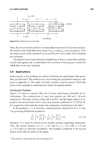
Figure 5.12. Reinforced concrete slab.

Thus, the correct velocity solution is indeed obtained earlier in the iteration process.

The last two rows in the table show values of p /p and p /p at convergence. They

m sm
are indeed small within round-off errors and become even smaller if the iterations
are continued.
The general lesson learnt from the example here is that, in a pure flow problem,
overall convergence rate is controlled by the evolution of the pressure variable for
which there is no exact equation.

5.6 Applications
In this section, a few problems are solved to illustrate the application of the proce-
dure just described. The problems are solved using the generalised computer code
given in Appendix C. The reader will find it useful to read the typical USER files
given in this appendix to understand the details of implementation.

Conduction Problem
Figure 5.12 shows a concrete slab with I-section steel beams embedded for re-
inforcement. The conductivities of steel and concrete are 100 and 1 W/m-K,
respectively. The lower surface of the slab is at 80 C and the upper surface is ex-
◦
2
posed to the environment at 20 C with a heat transfer coefficient of 1.75 W/m -K.
◦
It is required to determine the steady-state temperature distribution in the slab. 17
In this problem, u i = 0; therefore, solution need be obtained for = T only.
The governing differential equation is
∂ ∂T ∂ ∂T
K + K = 0. (5.115)
∂x 1 ∂x 1 ∂x 2 ∂x 2
Equation 5.115 must be solved on the smallest domain, exploiting symmetries.
Thus, the chosen domain is 0 ≤ x 1 ≤ 0.5 and 0 ≤ x 2 ≤ 1.0, with x 1 = 0 and
x 1 = 0.5 taken as symmetry boundaries. The boundary conditions at the top and
bottom of the slab are shown in the figure.

17 This problem is taken from the book by Patankar [53].