Page 162 - Introduction to Computational Fluid Dynamics

P1: IWV
0 521 85326 5
CB908/Date
0521853265c05
5.6 APPLICATIONS
L May 20, 2005 12:28 141
t
SYMMETRY
H A B C

PERIODIC PERIODIC

D
F E
SYMMETRY

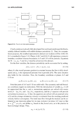
Figure 5.14. Flow in an interrupted passage.

Clearly, under periodically fully developed flow and heat transfer past the blocks,
suitably defined variables will exhibit distance periodicity 2L. Thus, for computa-
tional purposes, the smallest representative domain (or module) will be A-B-C-D-
E-F, as marked in Figure 5.14. Planes A-B-C and D-E-F will experience symmetry
boundary condition whereas boundaries A-F and C-D will be periodic. Equations
for = u 1 , u 2 , T and for p must be solved over this domain.

For the flow variables, the distance periodicity can be accounted for by setting
p (x 1 , x 2 ) =−β x 1 + p o (x 1 , x 2 ), (5.116)

where β is the overall pressure gradient (a constant because the flow is fully devel-
oped) and p o is the superposed pressure that is periodic [54]. The same situation
also holds for the velocities. Thus, the boundary conditions at planes A-F and
C-D are

p o (0, x 2 ) = p o (2L, x 2 ), u i (0, x 2 ) = u i (2L, x 2 ). (5.117)
Note that parts of A-F and C-D are solid walls. The symmetry and wall bound-
ary conditions require no elaboration. With the introduction of variable p o , it will
be appreciated that the u 1 and u 2 momentum equations are solved with source

terms β − ∂p o /∂x 1 and −∂p o /∂x 2 , respectively, and the p equation will provide
corrections to pressure p o . In fact, the equations are solved with an assumed value
of β and the average streamwise velocity is evaluated from the resulting predicted
velocity field at convergence. The total mass flow through the module can be es-
timated at any transverse plane but we may evaluate it at plane A-F (say) so that
H/2
˙ m = ρ u 1 dx 2 and define u av based on the frontal area, as is the practice in
0
heat-exchanger design. Thus,
u av = ˙ m/(ρ H/2). (5.118)