Page 161 - Introduction to Computational Fluid Dynamics

P1: IWV
12:28
May 20, 2005
CB908/Date
0521853265c05
140
1.0 0 521 85326 5 2D CONVECTION – CARTESIAN GRIDS
4
5 F 80.00
6
E 77.86
JB4 D 75.71
0.8 7
C 73.57
IB2 B 71.43
STEEL
JB3 A 69.29
0.6
9 67.14
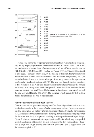
8 65.00 Figure 5.13. Isotherms – conduction in a re-
IB1 CONCRETE
7 62.86 inforced cement concrete slab.
0.4
6 60.71
JB2 5 58.57
4 56.43
8
JB1 3 54.29
0.2 9
A 2 52.14
B
C 1 50.00
D
E
0.0 F
0.25 0.5
Figure 5.13 shows the computed temperature contours. Computations were car-
ried out by employing harmonic-mean conductivities at the cell faces. This is im-
portant because conductivities of concrete and steel are different (see interfaces
IB1, IB2, JB1, JB2, JB3, and JB4 marked on Figure 5.13). A 13(x 1 ) × 22(x 2 ) grid
is employed. The figure shows that, in the middle of the slab, the temperature is
◦
almost uniform in both steel and concrete. The maximum temperature, 80 C, is
prescribed at the lower boundary and the predicted temperature at the top convec-
tive boundary is almost uniform at 54 C. The heat loss through the top boundary
◦
2
is thus calculated at 60 W/m and this also equals the heat gain through the bottom
boundary since steady-state conditions prevail. Note that if the I-section beams
were not present, one would have 1D heat conduction through concrete alone and
2
the heat loss would then be 38.2 W/m . The presence of high-conductivity I-section
beams has enhanced the rate of heat transfer.

Periodic Laminar Flow and Heat Transfer
Compact heat exchangers often employ an offset-fin configuration to enhance con-
vectiveheattransferattheexpenseofanincreasedpressuredrop.However,whenge-
ometric parameters are suitably chosen, the overall thermo-hydraulic performance
(i.e., increased heat transfer for the same pumping power or reduced pumping power
for the same heat duty) is improved, resulting in a compact heat exchanger design.
Figure 5.14 shows an array of interrupted plates or blocks, which may be regarded
as a 2D idealisation of the offset-fin heat exchanger; the flow width in the x 3 direc-
tion is large. The length and the width of each block are L and t, respectively, and
the transverse pitch is H.