Page 165 - Introduction to Computational Fluid Dynamics

P1: IWV
May 20, 2005
0 521 85326 5
CB908/Date
0521853265c05
12:28
144
TEMPERATURE
VELOCITY VECTORS 2D CONVECTION – CARTESIAN GRIDS
1.0 1.0 6 9 9 7 A
8
Re = 500 A 6
0.8 0.8 6
7 5
3 4 5
5 4
4
0.6 0.6 2 3 3
2
0.4 0.4 2 3
3 4 5 6
3 5 4 6
4
0.2 0.2
A 4
8 5
0.0 0.0 5 6
0.0 0.5 1.0 1.5 2.0 0.0 0.5 1.0 1.5 2.0
1.0 1.0 8
7
8
Re = 1000 5
0.8 0.8 A 5 6
9
3
3 5 4 7 6
4 4 5 4
3 3
0.6 0.6 2 2
2
0.4 0.4 2 3
3
4 4 6 5
5 3 4
6
5
0.2 0.2 5 4
9
7 6
8
0.0 0.0
0.0 0.5 1.0 1.5 2.0 0.0 0.5 1.0 1.5 2.0
1.0 1.0 5
9 A 6 7
4
Re = 2000
0.8 0.8
6
3 4 5 6 3 78 5
5 4
3 4 3
0.6 0.6 2 2
2
0.4 0.4 2
4 3 3 5 4
5 4 6
3 4 5 3
5
0.2 0.2 6
7
6 8
0.0 0.0
0.0 0.5 1.0 1.5 2.0 0.0 0.5 1.0 1.5 2.0
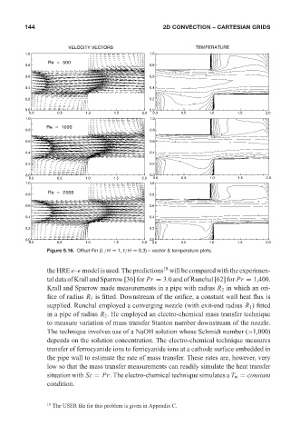
Figure 5.16. Offset Fin (L/H = 1, t/H = 0.3) – vector & temperature plots.
18
the HRE e– model is used. The predictions will be compared with the experimen-
tal data of Krall and Sparrow [36] for Pr = 3.0 and of Runchal [62] for Pr = 1,400.
Krall and Sparrow made measurements in a pipe with radius R 2 in which an ori-
fice of radius R 1 is fitted. Downstream of the orifice, a constant wall heat flux is
supplied. Runchal employed a converging nozzle (with exit-end radius R 1 ) fitted
in a pipe of radius R 2 . He employed an electro-chemical mass transfer technique
to measure variation of mass transfer Stanton number downstream of the nozzle.
The technique involves use of a NaOH solution whose Schmidt number (>1,000)
depends on the solution concentration. The electro-chemical technique measures
transfer of ferrocyanide ions to ferricyanide ions at a cathode surface embedded in
the pipe wall to estimate the rate of mass transfer. These rates are, however, very
low so that the mass transfer measurements can readily simulate the heat transfer
situation with Sc = Pr. The electro-chemical technique simulates a T w = constant
condition.
18 The USER file for this problem is given in Appendix C.