Page 170 - Introduction to Computational Fluid Dynamics

P1: IWV
CB908/Date
0 521 85326 5
0521853265c05
5.6 APPLICATIONS
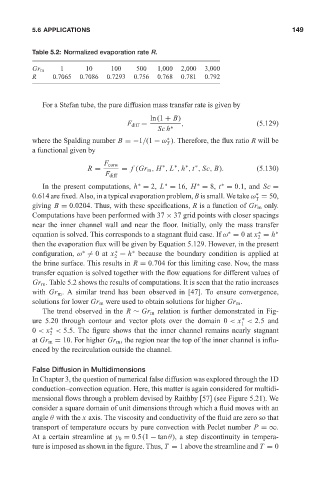
Table 5.2: Normalized evaporation rate R. May 20, 2005 12:28 149
Gr m 1 10 100 500 1,000 2,000 3,000
R 0.7065 0.7086 0.7293 0.756 0.768 0.781 0.792

For a Stefan tube, the pure diffusion mass transfer rate is given by
ln(1 + B)
F diff = , (5.129)
Sc h ∗
∗
where the Spalding number B =−1/(1 − ω ). Therefore, the flux ratio R will be
T
a functional given by
F conv
∗
∗
∗
∗
R = = f (Gr m , H , L , h , t , Sc, B). (5.130)
F diff
∗ ∗ ∗ ∗
In the present computations, h = 2, L = 16, H = 8, t = 0.1, and Sc =
0.614 are fixed. Also, in a typical evaporation problem, B is small. We take ω = 50,
∗
T
giving B = 0.0204. Thus, with these specifications, R is a function of Gr m only.
Computations have been performed with 37 × 37 grid points with closer spacings
near the inner channel wall and near the floor. Initially, only the mass transfer
equation is solved. This corresponds to a stagnant fluid case. If ω = 0at x = h ∗
∗
∗
2
then the evaporation flux will be given by Equation 5.129. However, in the present
∗
∗
configuration, ω = 0at x = h because the boundary condition is applied at
∗
2
the brine surface. This results in R = 0.704 for this limiting case. Now, the mass
transfer equation is solved together with the flow equations for different values of
Gr m . Table 5.2 shows the results of computations. It is seen that the ratio increases
with Gr m . A similar trend has been observed in [47]. To ensure convergence,
solutions for lower Gr m were used to obtain solutions for higher Gr m .
The trend observed in the R ∼ Gr m relation is further demonstrated in Fig-
ure 5.20 through contour and vector plots over the domain 0 < x < 2.5 and
∗
1
0 < x < 5.5. The figure shows that the inner channel remains nearly stagnant
∗
2
at Gr m = 10. For higher Gr m , the region near the top of the inner channel is influ-
enced by the recirculation outside the channel.
False Diffusion in Multidimensions
In Chapter 3, the question of numerical false diffusion was explored through the 1D
conduction–convection equation. Here, this matter is again considered for multidi-
mensional flows through a problem devised by Raithby [57] (see Figure 5.21). We
consider a square domain of unit dimensions through which a fluid moves with an
angle θ with the x axis. The viscosity and conductivity of the fluid are zero so that
transport of temperature occurs by pure convection with Peclet number P =∞.
At a certain streamline at y 0 = 0.5(1 − tanθ), a step discontinuity in tempera-
ture is imposed as shown in the figure. Thus, T = 1 above the streamline and T = 0