Page 175 - Introduction to Computational Fluid Dynamics

P1: IWV
0 521 85326 5
May 20, 2005
12:28
CB908/Date
0521853265c05
154
ζ
L 2D CONVECTION – CARTESIAN GRIDS

T = 0 L

η U

T = 1 Y0

T = 0
X0
T = 1
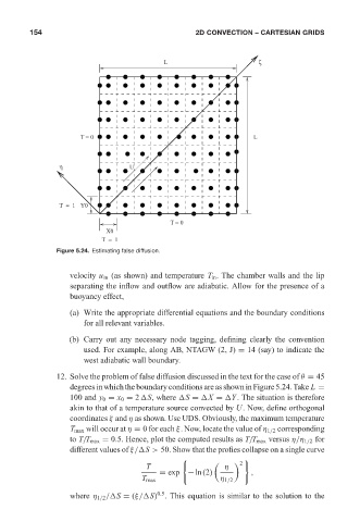
Figure 5.24. Estimating false diffusion.

velocity u in (as shown) and temperature T in . The chamber walls and the lip
separating the inflow and outflow are adiabatic. Allow for the presence of a
buoyancy effect,

(a) Write the appropriate differential equations and the boundary conditions
for all relevant variables.
(b) Carry out any necessary node tagging, defining clearly the convention
used. For example, along AB, NTAGW (2, J) = 14 (say) to indicate the
west adiabatic wall boundary.

12. Solve the problem of false diffusion discussed in the text for the case of θ = 45
degrees in which the boundary conditions are as shown in Figure 5.24. Take L =
100 and y 0 = x 0 = 2 S, where S = X = Y. The situation is therefore
akin to that of a temperature source convected by U. Now, define orthogonal
coordinates ξ and η as shown. Use UDS. Obviously, the maximum temperature
T max will occur at η = 0 for each ξ. Now, locate the value of η 1/2 corresponding
to T/T max = 0.5. Hence, plot the computed results as T/T max versus η/η 1/2 for
different values of ξ/ S > 50. Show that the profies collapse on a single curve
2
T η
= exp −ln(2) ,
T max η 1/2
0.5
where η 1/2 / S = (ξ/ S) . This equation is similar to the solution to the